In these eigenvalues and eigenvectors notes, we’ll review some results from linear algebra that are important for studying differential equations. Here, you will find the definitions and methods for finding eigenvalues and eigenvectors. We’ll also review some basic facts about systems of linear differential equations with constant coefficients, and walk through some examples of using the eigenvalues and eigenvectors for the solution.

What are the Eigenvalues and Eigenvectors?

Let \hat{A} be a square n \times n matrix, and a_{ij} be the elements of \hat{A} :

\hat{A} = \left(\begin{array}{cccc} a_{11} & a_{12} & \cdots& a_{1n} \ a_{21} & a_{22} & \cdots& a_{2n} \vdots& \vdots& \ddots& \vdots \ a_{m1} & a_{m2} & \cdots& a_{mn} \end{array} \right)

Matrix \hat{A} can be multiplied by a vector, \vec{xi} , with elements x_i:

\vec{xi} = \left(\begin{array}{c} x_{1} \ x_{2} \vdots \ x_{n} \end{array} \right)

The equation \hat{A}, \vec{xi} = \vec{y} can be considered a linear transformation that converts a vector, \vec{xi} , into a new vector, \vec{y} . Some vectors are transformed into multiples of themselves after such linear transformations. In this case, we have \vec{y} = \lambda \vec{xi} , where \lambda is a scalar proportionality factor. This situation, when the matrix \hat{A} acts by stretching or compressing some vector, without changing the direction of the vector, is illustrated in the following image:

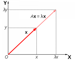
Matrix A stretches the vector x, and does not change its direction. By definition, such a vector x is an eigenvector of A.

To find such vectors, we seek solutions to the equation

\hat{A}, \vec{xi} = \lambda \vec{xi}

Values of \lambda that satisfy this equation are called the eigenvalues of the matrix \hat{A} , and we say that the vector \vec{xi} is an eigenvector belonging to the eigenvalue \lambda . The eigenvalue \lambda is allowed equal zero, but the eigenvectors \vec{xi} are, by definition, nonzero vectors.

Let’s illustrate eigenvalues and eigenvectors through a simple example.

Example 1

Let \hat{A} be a square n \times n matrix, and a_{ij} be the elements of \hat{A} :

We can check that

\hat{A},\vec{xi}_{(1)} = \left(\begin{array}{cc} 3 & -1 \ 4 & -2 \end{array} \right) \left(\begin{array}{c} 1 \ 1 \end{array} \right) = \left(\begin{array}{c} 2 \ 2 \end{array} \right) = 2\left(\begin{array}{c} 1 \ 1 \end{array} \right) = 2,\vec{xi}_{(1)}

and

\hat{A},\vec{xi}_{(2)} = \left(\begin{array}{cc} 3 & -1 \ 4 & -2 \end{array} \right) \left(\begin{array}{c} 1 \ 4 \end{array} \right) = \left(\begin{array}{c} -1 \ -4 \end{array} \right) = (-1)\left(\begin{array}{c} 1 \ 4 \end{array} \right) = (-1),\vec{xi}_{(2)}

It follows that \vec{xi}_{(1)} and \vec{xi}_{(2)} are eigenvectors of the matrix \hat{A} , corresponding to the eigenvalues \lambda_1 = 2 and \lambda_2 = -1 , respectively.

The Characteristic Equation

How can we determine the eigenvalues and eigenvectors for specific matrices? First, note that we can write the equation \hat{A}, \vec{xi} = \lambda \vec{xi} in the form

(\hat{A} - \lambda \hat{I} ) \vec{xi} = 0 ,, \qquad \text{where} \qquad \hat{I} = (\begin{array}{cccc} 1 & 0 & \cdots& 0 \ 0 & 1 & \cdots& 0 \vdots& \vdots& \ddots& \vdots \ 0 & 0 & \cdots& 1 \end{array} )

Here, we recognize a homogeneous system of linear algebraic equations for the components of the vector \vec{xi} . We know from linear algebra that such a system has nonzero solutions if and only if \lambda is chosen so that

det \left( \hat{A} - \lambda \hat{I} \right) = 0

The equation

det \left( \hat{A} - \lambda \hat{I} \right) = 0

is called the characteristic equation of a square matrix, \hat{A} .

The degree of the expression

det \left( \hat{A} - \lambda \hat{I} \right)

as a polynomial in \lambda is n , so there are n eigenvalues, \lambda_1, \lambda_2, \ldots, \lambda_n, which are all solutions of the characteristic equation. Some roots of this polynomial equation may be repeated. A root repeated k times is called an eigenvalue with multiplicity k . Further, the eigenvalue with multiplicity one is called simple. Any simple eigenvalue has at least one associated eigenvector. If all the eigenvalues of a matrix \hat{A} are simple, then the n eigenvectors of \hat{A} (one for each eigenvalue) are linearly independent. On the other hand, if \hat{A} has one or more repeated eigenvalues, then there may be fewer than n linearly independent eigenvectors. This is due to the fact that an eigenvalue of multiplicity k may have m < k linearly independent eigenvectors.

Let’s illustrate how we can use the characteristic equation to find eigenvalues and eigenvectors through examples.

Example 2

Find the eigenvalues and eigenvectors of the matrix

\hat{A} = \left(\begin{array}{cc} 5 & -1 \ 3 & 1 \end{array} \right)

The characteristic equation in this case takes the following form:

det \left( \hat{A} - \lambda \hat{I} \right) = 0 = det\left(\begin{array}{cc} 5 - \lambda & -1 \ 3 & 1 - \lambda \end{array} \right) = \lambda^2 - 6\lambda + 8 = (\lambda-2)(\lambda-4) = 0

The roots of this equation, \lambda_1 = 2 and \lambda_2 = 4 , are the eigenvalues of the matrix \hat{A} . To find the eigenvectors, we have to solve the equation \left( \hat{A} - \lambda \hat{I} \right) \vec{xi} = 0 with \lambda replaced by each of the eigenvalues. For \lambda = 2 , we have

\left(\begin{array}{cc} 3 & -1 \ 3 & -1 \end{array} \right) \left(\begin{array}{c} x_1 \ x_2 \end{array} \right) = \left(\begin{array}{c} 0 \ 0 \end{array} \right) ,, \qquad \text{or} \qquad 3x_1 - x_2 = 0

Hence, each row of this vector equation leads to the relation x_2 = 3 x_1 . If x_1 = C , then x_2 = 3C , and the eigenvector \vec{xi}_{(1)} corresponding to the eigenvalue \lambda_1 = 2 is

\vec{xi}_{(1)} = \left(\begin{array}{c} C \ 3C \end{array} \right) = C \left(\begin{array}{c} 1 \ 3 \end{array} \right),, \qquad C \neq 0

We can drop the arbitrary constant C when finding eigenvectors. Thus, we can write \vec{xi}_{(1)} = \left(\begin{array}{c} 1 \ 3 \end{array} \right) and remember that this vector multiplied by any nonzero number is also an eigenvector.

Now, setting \lambda = 4 , we obtain

\left(\begin{array}{cc} 1 & -1 \ 3 & -3 \end{array} \right) \left(\begin{array}{c} x_1 \ x_2 \end{array} \right) = \left(\begin{array}{c} 0 \ 0 \end{array} \right) ,, \qquad \text{or} \qquad x_1 - x_2 = 0

Thus, the eigenvector corresponding to the eigenvalue \lambda_2 = 4 is \vec{xi}_{(2)} = \left(\begin{array}{c} 1 \ 1 \end{array} \right) .

Example 3

Let’s investigate the eigenvalues and eigenvectors of the matrix

\hat{A} = \left(\begin{array}{cc} 2 & 1 \ 0 & 2 \end{array} \right)

Again, we start from the characteristic equation:

det\left( \hat{A} - \lambda \hat{I} \right) = 0 = det\left(\begin{array}{cc} 2 - \lambda & 1 \ 0 & 2 - \lambda \end{array} \right) = (2 - \lambda)^2 = 0

The solution to this equation, \lambda = 2 , is the eigenvalue, with multiplicity 2. The corresponding equation for eigenvectors takes the following form:

\left(\begin{array}{cc} 0 & 1 \ 0 & 0 \end{array} \right) \left(\begin{array}{c} x_1 \ x_2 \end{array} \right) = \left(\begin{array}{c} 0 \ 0 \end{array} \right) ,, \qquad \text{or} \qquad x_2 = 0

Notice that the vector component x_1 is free here, while x_2 is bound. We conclude that the matrix \hat{A} has only one eigenvector, \vec{xi} = \left(\begin{array}{c} 1 \ 0 \end{array} \right) , corresponding to the eigenvalue \lambda = 2 of multiplicity 2.

Example 4

Consider the following 3\times 3 matrix:

\hat{A} = \left(\begin{array}{ccc} 0 & 1 & 1 \ 1 & 0 & 1 \ 1 & 1 & 0 \end{array} \right)

Now, the eigenvalues are the roots of the following polynomial equation:

det ( \hat{A} - \lambda \hat{I} ) = det(\begin{array}{ccc} - \lambda & 1 & 1 \ 1 & - \lambda & 1 \ 1 & 1 & - \lambda \end{array} ) = - \lambda^3 + 3\lambda + 2 = -(\lambda - 2)(\lambda + 1)^2 = 0

Thus, \lambda_1 = 2 is a simple eigenvalue, and \lambda_2 = -1 is an eigenvalue of multiplicity 2. To find the eigenvector \vec{xi}_{(1)} corresponding to the eigenvalue \lambda_1 , we substitute \lambda = 2 into the equation \left( \hat{A} - \lambda \hat{I} \right) \vec{xi} = 0 . This gives the following vector equation:

\left(\begin{array}{ccc} -2 & 1 & 1 \ 1 & -2 & 1 \ 1 & 1 & -2 \end{array} \right) \left(\begin{array}{c} x_1 \ x_2 \ x_3 \end{array} \right) = \left(\begin{array}{c} 0 \ 0 \ 0 \end{array} \right)

This equation is satisfied if x_1 = x_2 = x_3 . Hence, we obtain the eigenvector

\vec{xi}_{(1)} = \left(\begin{array}{c} 1 \ 1 \ 1 \end{array} \right)

For the eigenvalue \lambda_2 = - 1 , we have the following equality:

\left(\begin{array}{ccc} 1 & 1 & 1 \ 1 & 1 & 1 \ 1 & 1 & 1 \end{array} \right) \left(\begin{array}{c} x_1 \ x_2 \ x_3 \end{array} \right) = \left(\begin{array}{c} 0 \ 0 \ 0 \end{array} \right) ,, \qquad \text{or} \qquad x_1 + x_2 + x_3 = 0

The values for two of the components among x_1, x_2, and x_3 can be chosen arbitrarily, while the third is determined from this equation. For example, we can take x_1 = 1 and x_2 = 0 . Then, x_3 = - 1 , and we have the following eigenvector:

\vec{xi}_{(2)} = \left(\begin{array}{c} 1 \ 0 \ -1 \end{array} \right)

The second linearly independent eigenvector can be found here by choosingother values for x_1 and x_2 . For instance, let x_1 = 0 and x_2 = 1 . Again, x_3 = - 1 , and we have the second eigenvector corresponding to the same eigenvalue , \lambda_2 = - 1 :

\vec{xi}_{(3)} = \left(\begin{array}{c} 0 \ 1 \ -1 \end{array} \right)

Therefore, in this example, we have three linearly independent eigenvectors associated with two eigenvalues, one with multiplicity 2.

Systems of Homogeneous Linear Differential Equations with Constant Coefficients

Consider a system of homogeneous linear differential equations with n unknown functions, y_1(t), y_2(t), \ldots, y_n(t) :

\begin{array}{c}\dot{y}_1 = a_{11} y_1 + a_{12} y_2 + \cdots + a_{1n} y_n \dot{y}_2 = a_{21} y_1 + a_{22} y_2 + \cdots + a_{2n} y_n \vdots \dot{y}_n = a_{n1} y_1 + a_{n2} y_2 + \cdots + a_{nn} y_n \end{array}) .

Here, a dot means differentiation with respect to the variable t . This system of differential equations can be presented in matrix form \dot{\vec{y}} = \hat{A},\vec{y} , if we define

\hat{A} = \left(\begin{array}{cccc} a_{11} & a_{12} & \cdots& a_{1n} \ a_{21} & a_{22} & \cdots& a_{2n} \ \vdots& \vdots& \ddots& \vdots \ a_{n1} & a_{n2} & \cdots& a_{nn} \end{array} \right) ,, \qquad \vec{y} = \left(\begin{array}{c} y_{1}(t) \ y_{2}(t) \vdots \ y_{n}(t) \end{array} \right)

We suppose that \hat{A} is a constant matrix. Then, the general solution of the differential equation \dot{\vec{y}} = \hat{A},\vec{y} can be presented in the following form:

\vec{y} = \vec{xi}, e^{\lambda t}

Here, the constant vector \vec{xi} and the exponent \lambda are to be determined from the equation

\lambda \vec{xi}, e^{\lambda t} = \hat{A},\vec{xi}, e^{\lambda t}

Upon canceling the nonzero scalar factor e^{\lambda t} , we obtain \hat{A},\vec{xi} = \lambda \vec{xi} , or

\left(\hat{A} - \lambda \hat{I} \right) \vec{xi} = 0

Here, again, \hat{I} is the n \times n identity matrix. This equation is precisely the one that determines the eigenvalues and eigenvectors of a matrix \hat{A} . Therefore, the vector \vec{y} that solves the system of homogeneous linear differential equations with constant coefficients can be presented in the form \vec{y} = \vec{xi},e^{\lambda t} , provided that \lambda is an eigenvalue and \vec{xi} is an associated eigenvector of the coefficient matrix \hat{A} .

If the eigenvalues of the matrix \hat{A} are all real and different, each eigenvalue, \lambda_i, is associated with a real eigenvector, \vec{xi}_{(i)} ,

and the eigenvectors

\vec{xi}_{(1)}, \vec{xi}_{(2)}, \ldots, \vec{xi}_{(n)}

are linearly independent. The corresponding general solution of the differential equation

\dot{\vec{y}} = \hat{A},\vec{y} is

\vec{y} = C_1 \vec{xi}_{(1)},e^{\lambda_1 t} + C_2 \vec{xi}_{(2)},e^{\lambda_2 t} + \cdots + C_n \vec{xi}_{(n)},e^{\lambda_n t}

Even if some of the eigenvalues are repeated, there can still be a full set of n  linearly independent eigenvectors,

\vec{xi}_{(1)}, \vec{xi}_{(2)}, \ldots, \vec{xi}_{(n)} .

It is only necessary to seek additional solutions of another form if the number of eigenvectors is smaller than n .

The following example illustrates this solution procedure.

Example 5

Consider the system of differential equations

\begin{array}{c}\dot{x} = y + z \dot{y} = x + z \dot{z} = x + y \end{array} .

This system can be presented in matrix form as follows:

\dot{\vec{y}} = \hat{A},\vec{y},, \qquad \text{where} \qquad \hat{A} = \left(\begin{array}{ccc} 0 & 1 & 1 \ 1 & 0 & 1 \ 1 & 1 & 0 \end{array} \right) ,, \qquad \vec{y} = \left(\begin{array}{c} x(t) \ y(t) \ z(t) \end{array} \right)

The eigenvalues and eigenvectors of the matrix \hat{A} were found in Example 4; namely,

\lambda_1 = 2 ,, \quad \lambda_2 = \lambda_3 = -1 ,, \qquad \vec{xi}_{(1)} = (\begin{array}{c} 1 \ 1 \ 1 \end{array} ) ,, \quad \vec{xi}_{(2)} = (\begin{array}{c} 1 \ 0 \ - 1 \end{array} ) ,, \quad \vec{xi}_{(3)} = (\begin{array}{c} 0 \ 1 \ - 1 \end{array} )

Hence, the general solution of the differential equation can be presented in the form

\vec{y} = C_1 \left(\begin{array}{c} 1 \ 1 \ 1 \end{array} \right)e^{2t} + C_2 \left(\begin{array}{c} 1 \ 0 \ - 1 \end{array} \right)e^{-t} + C_3 \left(\begin{array}{c} 0 \ 1 \ - 1 \end{array} \right)e^{-t}

Here, C_1 , C_2 , and C_3 are arbitrary constants of integration. Consequently, for the components of vector \vec{y} , we have

x(t) = C_1 e^{2t} + C_2 e^{-t} ,,\qquad y(t) = C_1 e^{2t} + C_3 e^{-t} ,,\qquad z(t) = C_1 e^{2t} - C_2 e^{-t} - C_3 e^{-t}

Thus, we have demonstrated how to use our knowledge of eigenvalues and eigenvectors of a matrix \hat{A} to determine the solution of the differential equation \dot{\vec{y}} = \hat{A},\vec{y} .

Wrapping Everything Up

In this eigenvalues and eigenvectors review article, we have investigated the eigenvalue problem in linear algebra, and have established its relationship with differential equations. Now, you will be able to find the eigenvalues and eigenvectors of a matrix with constant coefficients, and apply the result to the solution of linear differential equations. We hope this post addresses any confusion you might have had with eigenvalues and eigenvectors.

Featured Image Source

Looking for Differential Equations practice?

You can also find thousands of practice questions on Albert.io. Albert.io lets you customize your learning experience to target practice where you need the most help. We’ll give you challenging practice questions to help you achieve mastery in Differential Equations.

Start practicing here.

Are you a teacher or administrator interested in boosting Differential Equations student outcomes?

Learn more about our school licenses here.