What We Review
Differential equations appear in many areas of mathematics, especially on the AP® Calculus AB and BC exams. These equations relate a function to its derivatives, and they are tested under the topic FUN-7.A.1, which emphasizes understanding how functions connect to their rates of change. Therefore, a solid understanding of differential equations examples is crucial for exam success. This article discusses the basics of AP® Calculus AB differential equations in a step-by-step manner, covering the most important methods and contexts.
Introduction to Differential Equations
A differential equation is any equation involving a function and one or more of its derivatives. In simpler terms, it tells how a quantity changes based on that quantity’s current value or the value of other variables.
For example, population growth can be modeled with a differential equation that links the rate of change of the population to the current population itself. The solutions to these equations can be general or particular, depending on whether initial conditions are applied. Knowing how to solve and interpret these solutions prepares students for both AP® Calculus AB differential equations and more advanced college-level mathematics.
Fundamental Concepts of Differential Equations
A differential equation may be described by its order, which is the highest derivative present. If the equation includes the first derivative \frac{dy}{dx} but not higher derivatives, it is a first-order equation. The degree is the exponent of the highest derivative in its simplest form.
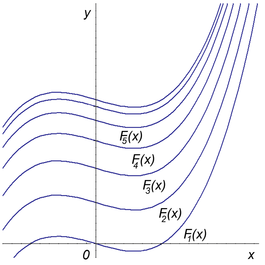
- A general solution includes a constant of integration because integration introduces an arbitrary constant. This can lead to an infinite number of solutions (as shown in the image below).
- A particular solution arises when an initial condition, such as y(x_0) = y_0, is used to find the specific value of that constant.
These ideas form the foundation of working with differential equations examples in AP® Calculus AB and BC.
Separable Differential Equations
Definition and Concept
A differential equation is said to be separable if it can be manipulated into a form resembling f(y)dy = g(x)dx. This means there is a way to write all the y terms on one side and all the x terms on the other side. After separating, integrating each side independently is straightforward.
Step-by-Step Example
Consider the differential equation \frac{dy}{dx} = \frac{2x}{3y}. Suppose there is an initial condition such as y(0) = 1. Follow these steps:
- Separate variables: \frac{dy}{dx} = \frac{2x}{3y}
- Multiply both sides by 3ydx: 3ydy = 2xdx.
- Integrate both sides: \int 3ydy = \int 2xdx.
- The left side becomes \frac{3y^2}{2}, and the right side becomes x^2.
- Thus, \frac{3y^2}{2} = x^2 + C, where C is the constant of integration.
- Solve for y: 3y^2 = 2x^2 + 2C.
- y^2 = \frac{2x^2}{3} + \frac{2C}{3}.
- Hence, y = \pm \sqrt{\frac{2x^2}{3} + \frac{2C}{3}}.
- Apply the initial condition y(0) = 1:
- When x = 0, y(0) = 1.
- Plug these values into y = \pm \sqrt{\frac{2x^2}{3} + \frac{2C}{3}}: 1 = \pm \sqrt{\frac{2(0)^2}{3} + \frac{2C}{3}}.
- Thus, 1 = \pm \sqrt{\frac{2C}{3}}.
- Choose the positive branch for consistency, so 1 = \sqrt{\frac{2C}{3}}.
- Squaring both sides gives 1 = \frac{2C}{3}.
- Therefore, C = \frac{3}{2}.
- Final particular solution: y = \sqrt{\frac{2x^2}{3} + \frac{2\cdot \frac{3}{2}}{3}} = \sqrt{\frac{2x^2}{3} + 1}.
Growth and Decay Problems
Explanation
Growth and decay problems illustrate how something changes proportionally to its current amount. For population growth, the rate of change of the population is proportional to the size of the population. For radioactive decay, the rate of change is proportional to the remaining quantity of a substance. Therefore, the differential equation often takes the form \frac{dy}{dt} = ky, where k is a constant of proportionality (positive for growth and negative for decay).
Step-by-Step Example
Consider the equation \frac{dy}{dt} = ky, with the initial condition y(0) = y_0. Here is how to solve it:
- Separate variables: \frac{dy}{y} = kdt.
- Integrate both sides: \int \frac{1}{y}dy = \int kdt.
- The left side becomes \ln|y|, and the right side is kt + C.
- So \ln|y| = kt + C.
- Solve for y:
- Exponentiate both sides: |y| = e^{kt + C} = e^C e^{kt}.
- Since e^C is just another constant, rename it as A = e^C.
- Thus, y = A e^{kt}.
- Apply the initial condition y(0) = y_0:
- When t = 0, y(0) = A e^{k \cdot 0} = A.
- Hence, A = y_0.
- Therefore, y = y_0 e^{kt}.
This formula describes both exponential growth (if k > 0) and decay (if k < 0).
Advanced Example: Modeling with a First-Order Differential Equation
Real-World Context
Many real-world situations, such as cooling processes or chemical mixing, can be represented with first-order differential equations. These models track how a variable changes based on differences in temperature or concentration.
Step-by-Step Example
Suppose a liquid in a container cools according to \frac{dT}{dt} = -k(T - T_{\text{env}}), where T is the temperature of the liquid, T_{\text{env}} is the constant ambient temperature, and k > 0 is a constant.
- Separate variables: \frac{dT}{T - T_{\text{env}}} = -kdt.
- Integrate both sides: \int \frac{1}{T - T_{\text{env}}} dT = \int -k dt.
- The left side becomes \ln|T - T_{\text{env}}|. The right side is -kt + C.
- Thus, \ln|T - T_{\text{env}}| = -kt + C.
- Solve for T:
- Exponentiate both sides: |T - T_{\text{env}}| = e^{-kt + C} = e^C e^{-kt}.
- Let A = e^C, so T - T_{\text{env}} = A e^{-kt}.
- Therefore, T = T_{\text{env}} + A e^{-kt}.
- Apply an initial condition as needed:
- For example, if the initial temperature at t = 0 is T(0) = T_0, thenT_0 = T_{\text{env}} + A e^0 = T_{\text{env}} + A.
- Hence, A = T_0 - T_{\text{env}}.
- So the particular solution is T = T_{\text{env}} + (T_0 - T_{\text{env}}) e^{-kt}.
Common Pitfalls and Tips
- Always include a constant of integration during indefinite integration.
- Therefore, check by differentiating the final answer to confirm correctness.
- Carefully separate variables so each variable remains on only one side of the equation.
- Watch for sign errors, which can be easy to make when rearranging terms.
Quick Reference Chart of Important Vocabulary and Definitions
| Term | Definition |
| Differential Equation | An equation that relates a function to one or more of its derivatives. |
| Separable Differential Equation | A differential equation that can be written as f(y)dy = g(x)dx. |
| Initial Condition | A value of the function at a specific point, used to find a unique solution. |
| General Solution | The family of solutions that includes an arbitrary constant of integration. |
| Particular Solution | The specific solution found by applying an initial condition to the general solution. |
| Rate of Change | The derivative of a function, often signifying how a quantity evolves over time. |
| Constant of Integration | The constant introduced through indefinite integration, denoted by C. |
| Order of a Differential Equation | The highest derivative appearing in the equation. |
Conclusion
Differential equations are a key part of AP® Calculus AB differential equations and AP® Calculus BC. By understanding how to express a function in terms of its derivatives, learners can work through classic scenarios like population growth and cooling processes. In every case, the steps involve separating variables (when possible), integrating, and applying initial conditions to find particular solutions.
The best way to gain confidence is to practice numerous differential equations examples. Whether the goal is to master FUN-7.A.1 or to prepare for advanced courses, careful study and repetition will develop the necessary skills.
Sharpen Your Skills for AP® Calculus AB-BC
Are you preparing for the AP® Calculus exam? We’ve got you covered! Try our review articles designed to help you confidently tackle real-world math problems. You’ll find everything you need to succeed, from quick tips to detailed strategies. Start exploring now!
Need help preparing for your AP® Calculus AB-BC exam?
Albert has hundreds of AP® Calculus AB-BC practice questions, free responses, and an AP® Calculus AB-BC practice test to try out.


