Exponential models with differential equations are powerful tools used throughout AP® Calculus AB-BC. They help explain how populations grow and how substances decay in real-world scenarios. These models appear almost everywhere, from biology to finance. Therefore, understanding how they work is essential.

Differential equations involve an unknown function and its derivatives. Specifically, exponential models with differential equations often rely on the idea that the rate of change is proportional to the quantity itself. This concept is central to exponential growth and decay problems.

AP® Calculus AB-BC learners often encounter these models when studying topics such as FUN-7.F.1, FUN-7.F.2, and FUN-7.G.1. Therefore, mastering exponential growth and decay helps ensure a solid foundation for other advanced calculus topics.

The Core Differential Equation

Meaning of \frac{dy}{dt} = k y

The expression \frac{dy}{dt} represents how fast a quantity y changes with respect to time t. Because this rate is proportional to y itself, there is a constant of proportionality called k.

• If k is positive, y grows exponentially.
• If k is negative, y decays exponentially.

This principle shows up in everyday contexts. For example, populations often grow faster when there are more individuals present. Likewise, radioactive substances decay faster when there is more material available.

Explanation of the Parameter k

The constant k signifies how quickly a quantity grows or shrinks:

• A positive k generates exponential growth.
• A negative k generates exponential decay.

Therefore, the sign and magnitude of k determine whether the function grows or shrinks, and how rapidly it does so.

General and Particular Solutions

General Solution

Solving the differential equation \frac{dy}{dt} = k y starts by separating variables. Then, integrating leads to the general solution:

y(t) = C e^{k t}

Here, C is the constant of integration. It can vary depending on initial conditions or other boundary conditions in the problem.

Particular Solutions Using Initial Conditions

Many exponential models require finding a particular solution that satisfies a condition like y(0) = y_{0}. By substituting t = 0 into the general solution, it follows that:

y(0) = C e^{k (0)} = C \times 1 = C

Therefore, C = y_{0}. This value shapes the curve so that it meets the exact situation defined by the problem.

Step-by-Step Example 1

A. Problem Statement

A population of bacteria grows exponentially. The rate of change of the population y satisfies:

\frac{dy}{dt} = 0.2 y

Initially, there are 100 bacterial cells at t = 0. Find the function y(t) that models this population.

Detailed Solution

1. Write the differential equation:
   • \frac{dy}{dt} = 0.2 y
2. Separate the variables and integrate:
   • \int \frac{1}{y} dy = \int 0.2 dt
   • \ln |y| = 0.2 t + C_1
3. Solve for y(t):
   • |y| = e^{0.2 t + C_1} = e^{C_1} e^{0.2 t}
   • Let C = e^{C_1}.
   • Thus, y(t) = C e^{0.2 t}
4. Apply the initial condition y(0) = 100:
   • y(0) = C e^{0.2 \times 0} = C = 100
   • Therefore, C = 100.
5. Present the particular solution:
   • y(t) = 100 e^{0.2 t}

Step-by-Step Example 2

Problem Statement

Consider a radioactive substance that decays exponentially with constant rate k = -0.05. The differential equation is:

\frac{dy}{dt} = -0.05 y

There are initially 500 grams of the substance. Find the function y(t) for this decay.

Detailed Solution

1. Identify the differential equation:
   • \frac{dy}{dt} = -0.05 y
2. Solve for the general solution:
   • Separate variables: \int \frac{1}{y} dy = \int -0.05 dt
   • Integrate: \ln |y| = -0.05 t + C_1|y| = e^{-0.05 t + C_1} = e^{C_1} e^{-0.05 t}
     • Let C = e^{C_1}. Hence, y(t) = C e^{-0.05 t}
3. Use the initial condition y(0) = 500:
   • y(0) = C e^{-0.05 \times 0} = C = 500
4. Show the particular solution:
   • y(t) = 500 e^{-0.05 t}

This result indicates exponential decay because k is negative.

VI. Important Insights and Tips

Interpreting Growth vs. Decay

• A positive k means exponential growth.
• A negative k means exponential decay.

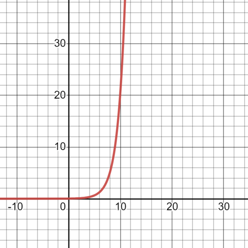
Therefore, checking the sign of k is essential before solving problems. Real-world applications might include population studies, finance (continuous compounding), and temperature change. The image below shows an example of exponential growth.

Common Pitfalls

• Forgetting the constant of integration C can lead to incorrect solutions.
• Mixing up growth and decay by accidentally assigning the wrong sign to k can create confusion.
• Omitting an initial condition leaves the solution incomplete, making it only a general solution.

Connection to Motion Along a Line (Optional Subtopic)

Models of velocity and acceleration sometimes draw on exponential relationships. While motion problems may involve other terms, growth and decay principles can occasionally come into play when describing rates of change proportional to the function.

Quick Reference Chart

Term	Definition
Exponential Model	A function that grows or decays proportionally to its size
Differential Equation	An equation involving a function and its derivatives
Rate of Change (\frac{dy}{dt})	The speed at which a quantity y changes with respect to t
Constant of Proportionality (k)	The factor measuring the rate of growth or decay
General Solution	A solution with an arbitrary constant C
Particular Solution	A solution determined by applying initial/boundary conditions

Conclusion

Exponential models with differential equations show how quantities change over time by linking their rate of change to their current size. The key equation \frac{dy}{dt} = k y captures both exponential growth (when k > 0) and exponential decay (when k < 0). Additionally, the constant of integration C adjusts the curve so that it meets specific initial conditions.

Reviewing these concepts often and working through examples will help develop strong calculus skills. Exploring more examples of exponential functions, including logistic growth and other real-life models, can deepen the understanding of exponential growth and decay beyond standard problems.

Sharpen Your Skills for AP® Calculus AB-BC

Are you preparing for the AP® Calculus exam? We’ve got you covered! Try our review articles designed to help you confidently tackle real-world math problems. You’ll find everything you need to succeed, from quick tips to detailed strategies. Start exploring now!

Need help preparing for your AP® Calculus AB-BC exam?

Albert has hundreds of AP® Calculus AB-BC practice questions, free responses, and an AP® Calculus AB-BC practice test to try out.