Taylor and Maclaurin series are crucial tools in AP® Calculus AB-BC. They help approximate complicated functions using simpler polynomials. Therefore, these series are often used to evaluate tricky limits, approximate integrals, and solve differential equations near a specific point. In particular, a Taylor polynomial approximates a function f(x) around x = a, while a Maclaurin series is a special case centered at x = 0. This review will explain the concepts behind taylor and maclaurin series, show when to use them, and provide taylor polynomial practice problems.
What We Review
Foundations of Taylor and Maclaurin Series
What Are Taylor Polynomials?
Taylor polynomials offer a way to approximate a function f(x) near x = a. They are formed by using the function’s derivatives at a. Specifically, the nth-degree Taylor polynomial for f(x) around x = a is:
[latex]P_n(x) = f(a) + \frac{f'(a)}{1!}(x - a) + \frac{f''(a)}{2!}(x - a)^2 + \dots + \frac{f^{(n)}(a)}{n!}(x - a)^n[/latex]Notice how the coefficient of each term depends on the nth derivative of f(x) evaluated at x = a. Moreover, these factorial denominators are crucial for getting correct coefficients.
What Is a Maclaurin Series?
A Maclaurin series is simply a Taylor series centered at a = 0. Therefore, it has the form:
[latex]P_n(x) = f(0) + \frac{f'(0)}{1!}x + \frac{f''(0)}{2!}x^2 + \dots + \frac{f^{(n)}(0)}{n!}x^n[/latex]This special case is often used for familiar functions such as e^x or trigonometric functions, making it a powerful tool in calculus.
Convergence and Approximation
Increasing Degree, Better Approximation
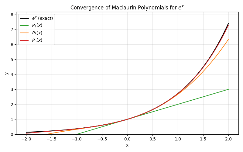
As the degree of a Taylor polynomial grows, the polynomial converges more closely to the actual function near x = a. In other words, adding more terms extends the interval where the polynomial provides an accurate approximation. However, some functions may require more terms than others to get the desired accuracy.
When to Use Taylor Polynomials for Approximation
Taylor polynomials are best suited for approximating function values near the center a. This aligns with the AP® Calculus concept of using expansions for local approximations. However, it is important to remember the interval of convergence. If x is too far from a, the polynomial may no longer give a good approximation. Thus, always check convergence conditions before relying on these expansions.
Constructing and Using Taylor Polynomials
Step-by-Step Procedure
- Identify the function f(x) and the point a about which you want to expand.
- Compute derivatives f'(x), f''(x), up to the nth derivative if needed.
- Evaluate each derivative at x = a.
- Plug these derivative values into the Taylor polynomial formula: P_n(x) = \sum_{k=0}^{n} \frac{f^{(k)}(a)}{k!}(x - a)^k
- Simplify the polynomial and check for any patterns.
Practical Tips and Common Mistakes
- Keep track of factorials carefully. Dividing by k! is a common place for errors.
- Be consistent with the sign of each term, especially for functions like \sin(x)
- Verify that derivative evaluations at a are correct. Even a small sign or numerical slip can derail the entire polynomial.
Examples with Step-by-Step Solutions
Example 1: Taylor Polynomial for e^x at a = 0
Consider f(x) = e^x. A Maclaurin series is used here.
- Derivatives:
- f(x) = e^x, \quad f'(x) = e^x, \quad f''(x) = e^x, \dots
- Evaluate at x = 0:
- f(0) = 1, f'(0) = 1, f''(0) = 1, \dots
- Construct the polynomial:
- P_n(x) = 1 + x + \frac{x^2}{2!} + \dots + \frac{x^n}{n!}
Therefore, the nth-degree Taylor (Maclaurin) polynomial for e^x is:
P_n(x) = \sum_{k=0}^{n} \frac{x^k}{k!}This polynomial approximates e^x especially well for values of x close to 0.
Example 2: Taylor Polynomial for \sin(x) at a = 0
Now look at f(x) = \sin(x).
- Derivatives:
- f(x) = \sin(x)
- Derivative: f'(x) = \cos(x)
- Second Derivative: f''(x) = -\sin(x)
- Third Derivative: f^{(3)}(x) = -\cos(x)
- Fourth Derivative: f^{(4)}(x) = \sin(x)
- Evaluate at x = 0:
- Function: f(0) = 0, \sin(0) = 0
- Derivative: f'(0) = 1, \cos(0) = 1
- Second Derivative: f''(0) = 0, -\sin(0) = 0
- Third Derivative: f^{(3)}(0) = -1, -\cos(0) = -1
- Fourth Derivative: f^{(4)}(0) = 0, \sin(0) = 0
- Construct the polynomial, including the pattern of alternating signs:
- P_n(x) \approx x - \frac{x^3}{3!} + \frac{x^5}{5!} - \dots
Thus, the Maclaurin series for \sin(x) includes only odd powers of x, with alternating signs.
Example 3: Taylor Polynomial for f(x) = (x - 2)^n Centered at a = 2
Consider f(x) = e^{x-2} if the goal is a function that naturally shifts the center to x = 2. (This is just one example of a function centered away from zero.)
- Let g(u) = e^u, where u = x - 2. Then f(x) = g(x - 2).
- For the Taylor expansion around x = 2, observe that f^{(n)}(2) = e^{2}. More precisely, each derivative of e^{x-2} evaluated at x = 2 yields e^0 = 1, but we must factor back in the shift if needed over multiple steps.
- Thus, the nth-degree Taylor polynomial around a = 2 becomes:
- P_n(x) = \sum_{k=0}^{n} \frac{f^{(k)}(2)}{k!}(x-2)^k
- Since f^{(k)}(2) = e^{0} = 1, the polynomial simplifies to:
- P_n(x) = 1 + (x - 2) + \frac{(x - 2)^2}{2!} + \dots + \frac{(x - 2)^n}{n!}
- That is exactly the shifted version of the Maclaurin series for e^x, but centered at 2.
VI. Quick Reference Chart
| Term | Definition or Key Feature |
| Taylor series | A polynomial expansion of f(x) around x = a |
| Maclaurin series | A special Taylor series centered at x = 0 |
| nth derivative | The nth order derivative of f(x), denoted by f^{(n)}(x) |
| Radius of convergence | The distance from a for which the series converges |
Conclusion
Taylor and Maclaurin series allow simpler polynomial approximations of more complex functions near a chosen point. By using higher-degree polynomials, it becomes possible to get more accurate approximations within a certain interval. It is essential to pay attention to factorial terms, signs, and the interval of convergence. These expansions come up often in AP® Calculus AB-BC, so consistent practice, such as doing taylor polynomial practice problems, is recommended. Mastering these series not only helps with exam preparation but also deepens understanding of how functions behave near a chosen value.
Sharpen Your Skills for AP® Calculus AB-BC
Are you preparing for the AP® Calculus exam? We’ve got you covered! Try our review articles designed to help you confidently tackle real-world math problems. You’ll find everything you need to succeed, from quick tips to detailed strategies. Start exploring now!
Need help preparing for your AP® Calculus AB-BC exam?
Albert has hundreds of AP® Calculus AB-BC practice questions, free responses, and an AP® Calculus AB-BC practice test to try out.


