Series play an important role in calculus. A power series is a sum of terms in the form of a_n(x - c)^n, where n is a nonnegative integer and c is the center. These series often represent functions that might otherwise be difficult to handle in exact form. Moreover, Taylor and Maclaurin series are especially important in AP® Calculus, because they offer a powerful way to approximate functions near certain points using tools like the Maclaurin series formula.

The purpose of this article is to explain the difference between Taylor and Maclaurin series. It will also show how to find and use the maclaurin series formula for common functions. Concepts such as the “cos x taylor polynomial,” “taylor polynomial for sin x,” and “cos x maclaurin series” will appear throughout the text.

Taylor Series vs. Maclaurin Series

Defining the Taylor Series

A Taylor series is an infinite sum of terms that represent a function near x = a. Each term comes from a Taylor polynomial, which is a partial sum of the full series. For a function f(x) that is infinitely differentiable at x = a, the Taylor series is:

\displaystyle f(x) = \sum_{n=0}^{\infty} \frac{f^{(n)}(a)}{n!}(x - a)^n

Here, f^{(n)}(a) is the n\text{th} derivative of f(x) evaluated at x = a. Therefore, the Taylor polynomials capture more and more detail of the function’s behavior as n grows.

The Maclaurin Series Formula

The maclaurin series formula is a special case of the Taylor series centered at x = 0. Instead of (x - a)^n, it uses simply x^n. Thus, the maclaurin series formula for f(x) is:

\displaystyle f(x) = \sum_{n=0}^{\infty} \frac{f^{(n)}(0)}{n!} x^n

This means that every term relies on derivatives evaluated at zero. Frequently used for functions like e^x, \sin x, and \cos x, it is quite useful for simplifying problems in calculus.

Why Maclaurin Series Matter

Maclaurin series are closely tied to well-known expansions, including e^x, \sin x, and \cos x. These expansions help approximate values of complicated functions, which can be valuable in physics, engineering, and beyond. In higher-level applications, one might use a finite number of terms as a partial sum to estimate a function’s value to a desired level of accuracy.

Common Maclaurin Series

Geometric Series for \frac{1}{1 - x}

A basic, yet essential, power series is the geometric series:

\displaystyle \frac{1}{1 - x} = \sum_{n=0}^{\infty} x^n

Its radius of convergence is |x| < 1. Therefore, within that interval, partial sums like 1 + x + x^2 + \ldots + x^N get closer to the actual value of \frac{1}{1 - x} as N increases.

Simple Demonstration of Partial Sums

Suppose x = 0.5. Then, the first few partial sums for \frac{1}{1 - x} are:

• 1
• 1 + 0.5 = 1.5
• 1 + 0.5 + 0.5^2 = 1.75
• 1 + 0.5 + 0.5^2 + 0.5^3 = 1.875

As the number of terms increases, the sum approaches \frac{1}{1 - 0.5} = 2.

Maclaurin Series for e^x, \sin x, and \cos x

Some of the most famous maclaurin expansions include:

• e^x = 1 + x + \frac{x^2}{2!} + \frac{x^3}{3!} + \cdots
• \sin x = x - \frac{x^3}{3!} + \frac{x^5}{5!} - \cdots
• \cos x = 1 - \frac{x^2}{2!} + \frac{x^4}{4!} - \cdots

Notice that the “taylor polynomial for sin x” and the “cos x maclaurin series” come directly from the maclaurin series formula by plugging in the derivatives of sine and cosine at zero.

Constructing a Taylor Polynomial for sin x and cos x

Finding the Taylor Polynomial for \sin x

To find the n\text{th} degree Taylor polynomial for \sin x around x = a, the derivatives of \sin x are plugged into the general formula. In particular, if it is centered at a = 0, the result is the Maclaurin version. These steps illustrate the process:

1. Compute derivatives:
   • f(x) = \sin x \quad \Rightarrow \quad f'(x) = \cos x
   • f''(x) = -\sin x
   • f^{(3)}(x) = -\cos x
   • f^{(4)}(x) = \sin x
2. Evaluate at x = 0:
   • \sin(0) = 0
   • \cos(0) = 1
   • -\sin(0) = 0, etc.
3. Plug into the Taylor formula.

Hence, the Maclaurin series is \sin x = x - \frac{x^3}{3!} + \frac{x^5}{5!} - \cdots.

Finding the Taylor Polynomial for \cos x

The steps are similar for \cos x. Repeated differentiation cycles through \cos x, -\sin x, -\cos x, and \sin x:

1. f(x) = \cos x \quad \Rightarrow \quad f'(x) = -\sin x
2. Evaluate at x=0:
   • \cos(0) = 1
   • -\sin(0) = 0
3. Insert these into the Maclaurin series formula to get:
   • \cos x = 1 - \frac{x^2}{2!} + \frac{x^4}{4!} - \cdots

That is the “cos x maclaurin series.” Meanwhile, a partial sum of that expansion can be called a cos x taylor polynomial centered at zero.

Examples with Step-by-Step Solutions

Example 1: Approximating e^x with a Taylor Polynomial

Demonstrate how to approximate e^x using a fourth-degree polynomial around x = 0:

1. Write out the series:
   • e^x = 1 + x + \frac{x^2}{2!} + \frac{x^3}{3!} + \frac{x^4}{4!} + \cdots
2. Take the partial sum using terms up to x^4:
   • P_4(x) = 1 + x + \frac{x^2}{2!} + \frac{x^3}{3!} + \frac{x^4}{4!}
3. If x = 1, then:
   • P_4(1) = 1 + 1 + \frac{1}{2!} + \frac{1}{3!} + \frac{1}{4!}.
4. Calculate numerically:
   • 1 + 1 + 0.5 + 0.1667 + 0.0417 \approx 2.7084.

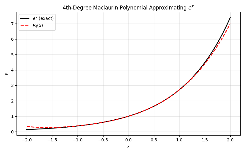
Compare this to e \approx 2.71828. The partial sum gets quite close to the true value with just a few terms.

Example 2: Finding a Third-Degree Maclaurin Polynomial for \sin x

Find the third-degree (i.e., up to x^3) Maclaurin polynomial:

1. List derivatives at x = 0:
   • \sin(0) = 0
   • \cos(0) = 1
   • -\sin(0) = 0
   • -\cos(0) = -1
2. Incorporate into the polynomial:
   • \sin x \approx x - \frac{x^3}{3!}.
3. Evaluate at x = \frac{\pi}{6} (30 degrees):
   • \sin\left(\frac{\pi}{6}\right) \approx \frac{\pi}{6} - \frac{\left(\frac{\pi}{6}\right)^3}{6}.
4. Simplify step by step:
   • \left(\frac{\pi}{6}\right)^3 = \frac{\pi^3}{216}
   • Divide by 6: \frac{\pi^3}{216 \times 6} = \frac{\pi^3}{1296}
   • Therefore, the approximation becomes \frac{\pi}{6} - \frac{\pi^3}{1296}, which is reasonably close to the exact value \frac{1}{2} once numerical values are used.

Quick Reference Chart

Term	Definition
Taylor Series	An infinite series of functions used to approximate a function around a specific point x = a.
Maclaurin Series	A special Taylor series centered at 0, often used for functions like e^x, \sin x, and \cos x.
Partial Sum	A finite portion (polynomial) of an infinite series used as an approximation of the full series.
Radius of Convergence	The set of x-values for which a power series converges to a finite value.
Geometric Series	A series with a constant ratio between successive terms.

Conclusion

Taylor and Maclaurin series remain pivotal in understanding how functions behave near specific points. The maclaurin series formula is simply a Taylor series centered at zero. Common examples like e^x, \sin x, and \cos x highlight how such expansions deliver powerful approximations.

In summary, these techniques are valuable for all sorts of higher-level calculus problems, including evaluating limits and solving differential equations. Future studies will explore convergence tests and more complex series, but the building blocks rest in the fundamentals of Taylor polynomials and their special case, the Maclaurin series.

Sharpen Your Skills for AP® Calculus AB-BC

Are you preparing for the AP® Calculus exam? We’ve got you covered! Try our review articles designed to help you confidently tackle real-world math problems. You’ll find everything you need to succeed, from quick tips to detailed strategies. Start exploring now!

Need help preparing for your AP® Calculus AB-BC exam?

Albert has hundreds of AP® Calculus AB-BC practice questions, free responses, and an AP® Calculus AB-BC practice test to try out.