Have you noticed that a phone battery seems to drop at a steady pace, while popular posts gain likes faster and faster? One drops linearly; the other rises exponentially. The SAT® loves to test this difference. Therefore, knowing how to spot, build, and compare growth models can lift your score. This guide breaks the topic into small, friendly steps so you can master every question on linear and exponential growth​.

Why Growth Models Matter on the SAT®

The SAT® Math section often asks you to:

• Choose the best model for a data set
• Read and interpret graphs or tables
• Use a model to predict future values

Because of this, a strong grip on linear and exponential growth means quick points. Next, discover how these two models differ.

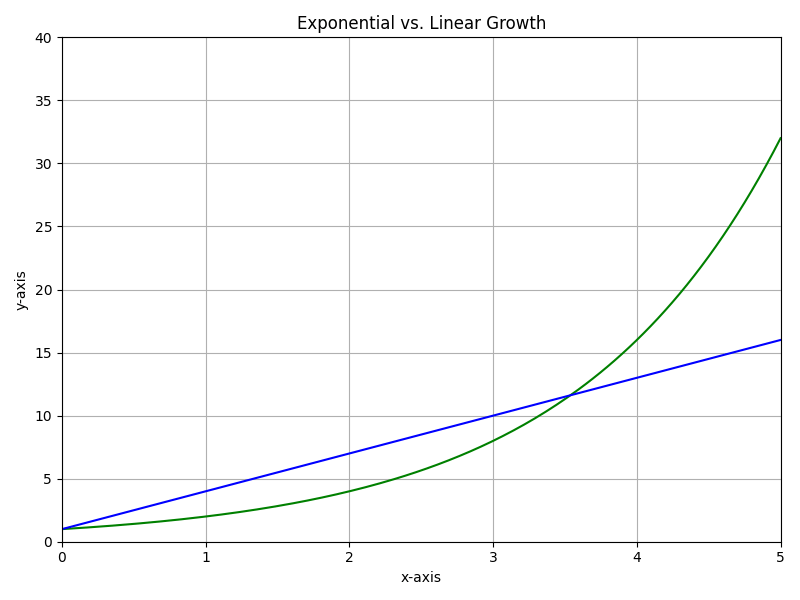
Linear vs. Exponential Growth

Key Ideas

• Linear growth: adds the same amount each step.
  • Pen-and-paper analogy: stacking one penny at a time.
• Exponential growth: multiplies by the same factor each step.
  • Biology analogy: bacteria that double every hour.

Mini Comparison Table

Feature	Linear	Exponential
Formula	y = mx + b	y = a\cdot b^{x}
Pattern	Constant difference	Constant ratio
Graph shape	Straight line	A curve that grows or shrinks faster and faster

If the gap between outputs stays equal, think linear. However, if the ratio stays equal, think exponential.

Building the Models from Scratch

Linear Model Essentials

• Slope-intercept form: y = mx + b
• Slope m: change in y for each 1-unit change in x.
• y-intercept b: value of y when x = 0.

Exponential Model Essentials

• General form: y = a\cdot b^{x}
• Initial value a: starting amount when x = 0.
• Growth/decay factor b:
  • If b > 1, growth.
  • If 0 < b < 1, decay.

Example 1

Two College-Savings Plans

Plan A adds \$1500 each year. Plan B starts at \$1000 and grows by 8\% per year.

1. Write Plan A.

• Slope m = 1500.
• Intercept b = 0 (start at \$0).
• Model: y = 1500x.

2. Write Plan B.

• Initial value a = 1000.
• Growth factor b = 1 + 0.08 = 1.08.
• Model: y = 1000\cdot 1.08^{x}.

3. Compare after 5 years.

• Plan A: y = 1500(5) = 7500.
• Plan B: y = 1000\cdot 1.08^{5}\approx 1469.

Therefore, at 5 years, the linear plan leads. However, the exponential plan will eventually overtake because multiplication beats addition in the long run.

Practice Problem

Write a model for a car that depreciates 12\% per year from \$25{,}000.

Solution: y = 25000\cdot 0.88^{x}.

Reading Graphs and Tables Quickly

A quick glance tells a lot.

• Straight-line graph → linear.
• Curved and getting steeper → exponential growth.
• Curved and flattening → exponential decay.

Interpreting Key Elements

• Slope: A steeper line means a larger change per unit.
• y-intercept: starting value.
• Key points: ordered pairs like (2, 5) give real-world snapshots.

Example 2

A graph shows a line passing through (0, 20) and (4, 36).

1. Compute slope: m = \frac{36 - 20}{4 - 0} = 4.
2. Equation: y = 4x + 20.
3. Interpretation: “The quantity begins at 20 and increases by 4 units per time period.”

Scatterplots and the Line of Best Fit

SAT® Math may provide a cloud of points and ask for the line of best fit.

Estimating Slope and Intercept by Hand

1. Draw a straight line that balances points above and below.
2. Pick two convenient points on that line, not necessarily data points.
3. Use them to find slope m and intercept b.

Technology Tip

When calculators are allowed, use the LinReg function to find m, b, and the correlation coefficient r.

Example 3

In the scatterplot below, points roughly cluster along a line. Two good points on the visual fit are (2, 5) and (8, 17). What is a good estimation for x=10?

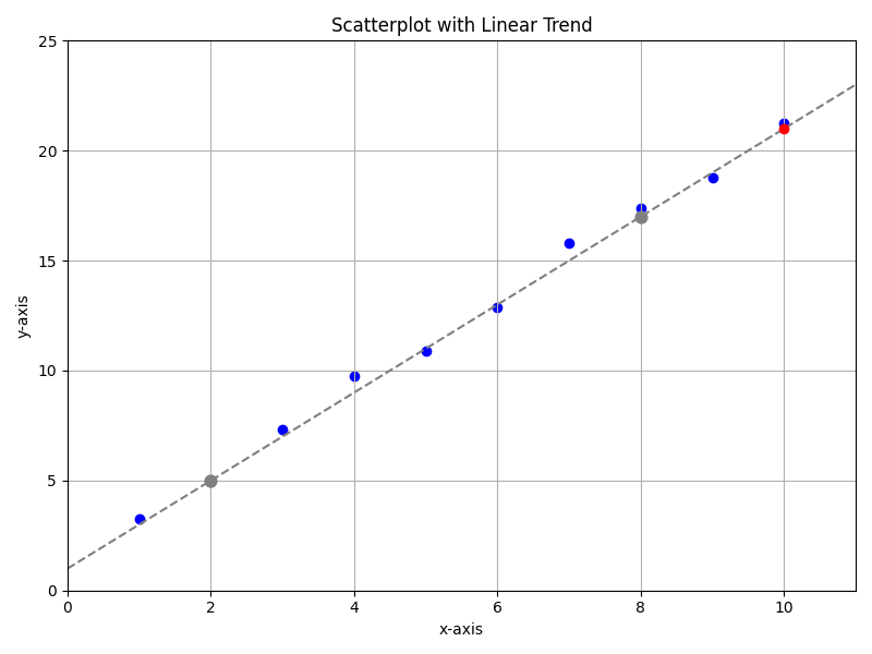
1. Slope: m = \frac{17 - 5}{8 - 2} = 2.
2. Intercept: Plug (2, 5) into y = 2x + b. Thus 5 = 2(2) + b \Rightarrow b = 1.
3. Model: y = 2x + 1.
4. Predict at x = 10: y = 2(10) + 1 = 21.

Therefore, about 21 is a reasonable forecast.

Practice Problem

Given a line of best fit y = 0.5x + 6, estimate y when x = 12.

Solution: y = 0.5(12) + 6 = 12.

Choosing the Best Model for Data Sets

First Differences vs. Common Ratios

• Create a table of outputs.
• First difference = subtract consecutive outputs.
  • Constant → linear.
• Common ratio = divide consecutive outputs.
  • Constant → exponential.

Residuals and Correlation Coefficient (Light Overview)

• Residual: actual minus predicted. Smaller residuals → better fit.
• Correlation coefficient r: close to 1 or –1 means a strong linear relationship.

Example 4

Sales per quarter: 20, 24, 28, 32.

1. Differences: 4, 4, 4. These are contstant; therefore, the relationship is linear.
2. A ratio check is not needed since the relationship is linear.
3. Linear model: y = 4x + 16.

Practice Problem

Data: 5, 7.5, 11.25, 16.875. Decide on the model type.

Solution: Ratios are 1.5 each time → exponential.

Comparing Predictions and Avoiding Extrapolation Traps

Using models to forecast is powerful; however, danger lurks beyond the data range.

• Linear predictions can under-estimate long-term exponential growth.
• Exponential predictions can skyrocket unrealistically when applied too far out.

Example 5

A population starts at 100 organisms.

• Model A: y = 20x + 100
• Model B: y = 100\cdot 1.15^{x}

1. At x = 3 days:

• Linear: y = 20(3) + 100 = 160.
• Exponential: y = 100\cdot 1.15^{3}\approx 152.

2. At x = 10 days:

• Linear: y = 20(10) + 100 = 300.
• Exponential: y = 100\cdot 1.15^{10}\approx 404.

Therefore, the exponential model soon surpasses the linear one. Do not assume the lower early value stays lower later.

Practice Problem

Which model likely fits compound interest?

Solution: Exponential, because money grows by a percentage.

SAT® Math Tips & Common Pitfalls

• Always label units; mix-ups cost points.
• Check the scale on axes; sometimes each square is 5, not 1.
• If ratios keep changing slightly, still test exponential on the calculator.
• Avoid extrapolating way beyond the data unless the test clearly allows it.
• On scatterplots, choose “best fit” lines that balance above and below points.
• When answers list forms, match exactly: slope-intercept vs. point-slope.
• Use calculator shortcuts: STO→ for fast table creation, LinReg for best fit.
• Eliminate answer choices with impossible y-intercepts (e.g., negative height).

Quick Reference Vocabulary Chart

Term	Concise Definition or Key Feature
Slope m	Rate of change; rise over run in y = mx + b
y-intercept b	Output when x = 0
Growth factor b	Multiplier in y = a\cdot b^{x}
Line of best fit	A straight line that models a scatterplot with minimal total residuals
Residual	Actual minus predicted value
Extrapolation	Predicting outside the data range
First difference	Consecutive subtraction to test linearity
Common ratio	Consecutive division to test exponentiality
Correlation coefficient r	Measures strength of linear relationship, –1 ≤ r ≤ 1
Constant difference	Fixed amount added each step; signals linear growth

Conclusion and Next Steps

Linear and exponential growth questions may look tricky, yet they follow clear patterns. Because you now know how to:

• Recognize each model
• Build equations from data
• Compare predictions

…SAT® Math traps should feel less scary. Therefore, keep practicing timed drills: glance at a table, decide the model, and write its equation in under one minute. With consistent effort, every linear or exponential question will feel like a free point.

Good luck and happy studying!

Sharpen Your Skills for SAT® Math (Digital)

Are you preparing for the SAT® Math (Digital) test? We’ve got you covered! Try our review articles designed to help you confidently tackle real-world SAT® Math (Digital) problems. You’ll find everything you need to succeed, from quick tips to detailed strategies. Start exploring now!

Need help preparing for your SAT® Math (Digital) exam?

Albert has hundreds of SAT® Math (Digital) practice questions, free response, and full-length practice tests to try out.