Limits are a key part of calculus, helping students understand how functions behave as inputs get closer and closer to specific values. In many cases, estimating the limit numerically provides helpful insight before learning more advanced methods. Indeed, the College Board’s AP® Calculus AB-BC Review mentions LIM-1.C.5, which highlights using numerical information to find a good approximation for a limit. Therefore, having a solid grasp of how to estimate the limit numerically is valuable for building problem-solving skills and confidence.

What Does It Mean to Estimate the Limit Numerically?

A limit expresses the behavior of a function as the input approaches a certain point. Though the function might not be defined at that point, it often settles near a specific number. Numerical estimation comes in handy when algebraic approaches become tricky.

To estimate the limit numerically, one might test values close to the point of interest. By observing how the output (the function value) behaves, the limiting value often emerges. This method bridges the gap between purely theoretical understanding and a hands-on approach.

Example 1: Simple Limit Demonstration

Consider the function f(x) = x^2 - 4. Suppose the task is to estimate the limit as x approaches 2.

Step-by-step solution:

1. Identify the point of interest: x = 2.
2. Substitute values close to 2, such as 1.9 and 2.1.
   • f(1.9) = (1.9)^2 - 4 = 3.61 - 4 = -0.39.
   • f(2.1) = (2.1)^2 - 4 = 4.41 - 4 = 0.41.
3. Notice that as x moves closer to 2, the outputs hover near 0.
4. Conclude that the limit appears to be 0.

Practice Problem for Example 1:

Estimate the limit of g(x) = 3x - 6 as x approaches 2 by evaluating at least two numbers close to 2.

Step-by-step solution (practice problem):

1. Identify the inputs near 2, such as 1.9 and 2.1.
2. Evaluate the function:
   • g(1.9) = 3(1.9) - 6 = 5.7 - 6 = -0.3.
   • g(2.1) = 3(2.1) - 6 = 6.3 - 6 = 0.3.
3. Observe that both values are close to 0, suggesting the limit is 0.

Common Methods for Numerical Limit Estimation

Direct Substitution

Direct substitution means plugging the point of interest directly into the function. When the function is defined at that point and no special complications arise, the result gives the limit. However, this technique fails if there is a division by zero or another undefined situation at that input.

Table of Values (T-Chart Method)

Another reliable strategy is setting up a small table of values (a T-chart). By choosing x-values slightly less than and slightly greater than the point, it becomes easier to see the trend in function outputs. This T-chart method helps avoid possible mistakes from one or two random guesses.

Approaching From Left and Right

Sometimes a function behaves differently when approaching from the left side (negative direction) compared to the right side (positive direction). For a limit to exist, both the left-hand limit and right-hand limit should agree. Consequently, checking from both directions is crucial.

Example 2: Table of Values Method

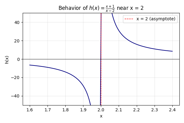
Estimate the limit of h(x) = \frac{x + 1}{x - 2} as x approaches 2.

Step-by-step solution:

1. Recognize that direct substitution at x = 2 fails because the denominator becomes 0.
2. Create a small table of values around 2, such as 1.9, 1.99, 2.01, and 2.1.
   • h(1.9) = \frac{1.9 + 1}{1.9 - 2} = \frac{2.9}{-0.1} = -29.
   • h(1.99) = \frac{1.99 + 1}{1.99 - 2} \approx \frac{2.99}{-0.01} = -299.
   • h(2.01) = \frac{2.01 + 1}{2.01 - 2} = \frac{3.01}{0.01} = 301.
   • h(2.1) = \frac{2.1 + 1}{2.1 - 2} = \frac{3.1}{0.1} = 31.
3. Observe that from the left side, the values become very large negative numbers, while from the right side, they become very large positive numbers. Thus, there is a vertical asymptote at x = 2, indicating the limit does not exist in a finite sense.

Practice Problem for Example 2:

Use a short table of values to estimate the limit of p(x) = \frac{1}{x - 3} as x approaches 3.

Step-by-step solution (practice problem):

1. Pick values near 3, such as 2.9 and 3.1.
2. Calculate the outputs:
   • p(2.9) = \frac{1}{2.9 - 3} = \frac{1}{-0.1} = -10.
   • p(3.1) = \frac{1}{3.1 - 3} = \frac{1}{0.1} = 10.
3. Notice the output shoots down to large negative values from the left, and up to large positive values from the right. Therefore, the limit as x approaches 3 does not exist as a finite number.

Recognizing Potential Pitfalls

Even an experienced problem solver must watch out for rounding errors, forgetting to check both sides, or missing the possibility that the limit does not exist. A function might oscillate indefinitely near the point of interest, or it may behave differently from the left than from the right.

Example 3: Trickier Function with Indeterminate Form

Consider q(x) = \frac{x^2 - 25}{x - 5} and estimate the limit as x approaches 5.

Step-by-step solution:

1. Notice direct substitution results in \frac{0}{0}, an indeterminate form.
2. Choose numbers around 5, such as 4.9 and 5.1.
   • q(4.9) = \frac{(4.9)^2 - 25}{4.9 - 5} = \frac{24.01 - 25}{-0.1} = \frac{-0.99}{-0.1} = 9.9.
   • q(5.1) = \frac{(5.1)^2 - 25}{5.1 - 5} = \frac{26.01 - 25}{0.1} = \frac{1.01}{0.1} = 10.1.
3. From these computations, the function seems to hover near 10. A more refined check with values like 4.99 or 5.01 would strengthen this conclusion.

Practice Problem for Example 3:

Estimate the limit of r(x) = \frac{x^2 - 16}{x - 4} as x approaches 4, using two numbers close to 4.

Step-by-step solution (practice problem):

1. Identify the indeterminate form when x = 4.
2. Pick values near 4, such as 3.9 and 4.1.
   • r(3.9) = \frac{(3.9)^2 - 16}{3.9 - 4} = \frac{15.21 - 16}{-0.1} = \frac{-0.79}{-0.1} = 7.9.
   • r(4.1) = \frac{(4.1)^2 - 16}{4.1 - 4} = \frac{16.81 - 16}{0.1} = \frac{0.81}{0.1} = 8.1.
3. Conclude that the limit appears to be near 8.

Additional Tips for Accurate Numerical Estimation

• Use smaller increments. Narrow intervals around the point make the estimate more reliable.
• Observe consistency. If outputs from both sides align with each other, this lends credibility to the estimated limit.
• Verify results with approximate calculations, especially when answers appear counterintuitive.

Example 4: Refining the Estimate

Suppose estimation is needed for s(x) = \frac{2x}{\sqrt{x + 4}} as x approaches 0.

Step-by-step solution:

1. Start with coarse values near 0, such as -0.5 and 0.5.
   • s(-0.5) = \frac{2(-0.5)}{\sqrt{-0.5 + 4}} = \frac{-1}{\sqrt{3.5}} \approx -0.5345.
   • s(0.5) = \frac{2(0.5)}{\sqrt{0.5 + 4}} = \frac{1}{\sqrt{4.5}} \approx 0.4714.
2. Narrow the gap by using -0.1 and 0.1.
   • s(-0.1) \approx \frac{-0.2}{\sqrt{3.9}} \approx -0.1013.
   • s(0.1) \approx \frac{0.2}{\sqrt{4.1}} \approx 0.0989.
3. Note that as x gets closer to 0, outputs focus near 0. Thus, the limit is 0.

Practice Problem for Example 4:

Refine the limit estimation of t(x) = \frac{x - 1}{\sqrt{x + 2}} as x approaches -1 by using smaller and smaller increments.

Step-by-step solution (practice problem):

1. Begin with x = -1.1 and x = -0.9.
   • t(-1.1) = \frac{-1.1 - 1}{\sqrt{-1.1 + 2}} = \frac{-2.1}{\sqrt{0.9}} \approx \frac{-2.1}{0.9487} \approx -2.21.
   • t(-0.9) = \frac{-0.9 - 1}{\sqrt{-0.9 + 2}} = \frac{-1.9}{\sqrt{1.1}} \approx \frac{-1.9}{1.0488} \approx -1.81.
2. Move closer with x = -1.01 and x = -0.99.
   • t(-1.01) \approx \frac{-2.01}{\sqrt{0.99}} \approx \frac{-2.01}{0.99499} \approx -2.02.
   • t(-0.99) \approx \frac{-1.99}{\sqrt{1.01}} \approx \frac{-1.99}{1.00499} \approx -1.98.
3. Conclude the limit hovers near -2.

VI. Quick Reference Chart

Term	Definition
Limit	The value a function approaches as the input nears a certain point, even if the function is not defined at that point.
Numerical Estimation of a Limit	Approximating a limit by evaluating the function at values close to the point in question.
Left-Hand Limit	The limit value approached as x approaches a point from the left.
Right-Hand Limit	The limit value approached as x approaches a point from the right.
T-Chart (Table of Values)	A strategy for estimating a limit by listing x-values near the point and observing the resulting function outputs.

Conclusion

Estimating the limit numerically is a practical skill that complements formal algebraic methods. Direct substitution, the table of values approach, and checking from both sides each provide clues about a function’s behavior. Indeed, practice reduces errors, and using smaller increments assures more precise estimates. Finally, a thorough understanding builds intuition about whether a limit exists—and, if it does, where it is heading. Therefore, keep exploring these strategies, and build confidence by testing different functions around challenging points.

Sharpen Your Skills for AP® Calculus AB-BC

Are you preparing for the AP® Calculus exam? We’ve got you covered! Try our review articles designed to help you confidently tackle real-world math problems. You’ll find everything you need to succeed, from quick tips to detailed strategies. Start exploring now!

Need help preparing for your AP® Calculus AB-BC exam?

Albert has hundreds of AP® Calculus AB-BC practice questions, free responses, and an AP® Calculus AB-BC practice test to try out.