Differential equations are equations that include a function and its derivative. They appear in many real-world settings, such as population growth and physics. However, exact solutions to these equations are not always easy to find. Therefore, numerical approximations, such as Euler’s method, can be helpful in AP® Calculus AB-BC.
Euler’s Method is a popular way to approximate solutions to differential equations. It works by estimating the slope and then stepping forward in small increments. This approach is especially useful when finding an exact formal solution is challenging. Many practical problems use this method to predict behavior, such as changes in temperature or the motion of an object.
What We Review
Understanding Euler’s Method
Basic Idea Behind Euler’s Method
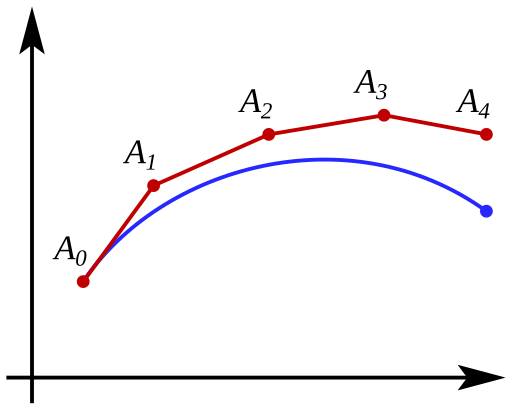
Euler’s Method starts with a known point on a curve and uses the slope from a differential equation to move step by step. Each step applies a small change in the x-direction, called \Delta x, to find a new approximate y-value. This process continues until reaching the region of interest. The general theory behind this can be seen in the visual below.
Key reasons for using this iterative process include:
- It builds from a simple slope estimate at each step.
- It allows for smaller step sizes to improve accuracy.
- It helps when new points cannot be found using an exact formula.
Key Formula
The main formula for Euler’s Method is:
y_{n+1} = y_n + f(x_n, y_n)\Delta xHere:
- x_n is the current x-value.
- y_n is the current y-value.
- \Delta x is the chosen step size.
- f(x_n, y_n) is the slope from the differential equation evaluated at the point (x_n, y_n).
This formula ensures the next approximation y_{n+1} is found by adding the slope times the step size to the current y-value.
Step-by-Step Example
Example Setup
Consider the differential equation \frac{dy}{dx} = 2x - y, with an initial condition of y(0) = 1. Suppose the step size \Delta x = 0.1. The goal is to find approximate values of y for a few steps using Euler’s Method.
Calculation Process
- Start at x_0 = 0 and y_0 = 1.
- Calculate the slope from the differential equation: f(x_0, y_0) = 2(0) - 1 = -1.
- Multiply the slope by \Delta x: \text{slope} \times \Delta x = -1 \times 0.1 = -0.1.
- Find the next y-value: y_{1} = y_{0} + (-0.1) = 1 + (-0.1) = 0.9.
- Increase x by the step size: x_1 = x_0 + 0.1 = 0.1.
Repeat these steps for a couple more iterations:
- Second iteration:
- f(x_1, y_1) = 2(0.1) - 0.9 = 0.2 - 0.9 = -0.7
- y_2 = y_1 + (-0.7 \times 0.1) = 0.9 - 0.07 = 0.83
- x_2 = x_1 + 0.1 = 0.2
- Third iteration:
- f(x_2, y_2) = 2(0.2) - 0.83 = 0.4 - 0.83 = -0.43
- y_3 = y_2 + (-0.43 \times 0.1) = 0.83 - 0.043 = 0.787
- x_3 = x_2 + 0.1 = 0.3
Conclusion from the Example
After three steps, the approximate value of y at x = 0.3 is 0.787. Note that the method’s accuracy often increases if the step size is smaller. However, too small a step size can mean more computations, so there is a balance to consider.
Additional Example with a Different Step Size
Using the Same Equation for Comparison
To see how step size impacts accuracy, revisit the same differential equation: \frac{dy}{dx} = 2x - y. This time, choose a bigger step size, \Delta x = 0.2, but keep the same initial condition y(0) = 1.
Step-by-Step Process
- At x_0 = 0, y_0 = 1.
- f(0, 1) = 2(0) - 1 = -1
- y_1 = y_0 + (-1 \times 0.2) = 1 - 0.2 = 0.8
- x_1 = 0.2
- At x_1 = 0.2, y_1 = 0.8.
- f(0.2, 0.8) = 2(0.2) - 0.8 = 0.4 - 0.8 = -0.4
- y_2 = 0.8 + (-0.4 \times 0.2) = 0.8 - 0.08 = 0.72
- x_2 = 0.4
Notice that this approximate solution shows bigger jumps and might lack the finer accuracy of a smaller \Delta x. However, it reaches a further x-value faster.
Observations
The accuracy of Euler’s Method is affected by step size. A smaller step size leads to more precise results but requires more calculating. Large step sizes may save time, but can stray from the true solution. An Euler’s Method calculator can handle many steps quickly, although understanding each step by hand is crucial during exams and practice.
Common Pitfalls and Tips for Success
- Keep the step size \Delta x consistent throughout the calculations.
- Watch for rounding errors, especially when doing manual work.
- Check that the initial condition is applied correctly before proceeding.
- Always consider whether the approximations seem reasonable by looking at the sign of the slope.
- Recognize that Euler’s Method outcomes will be closer to the exact solution when \Delta x is small, but that also means more steps.
Quick Reference Chart
Below is a helpful chart of important vocabulary and definitions for Euler’s Method:
| Term | Definition |
| Differential Equation | An equation involving a function and its derivative or derivatives. |
| Initial Value or Condition | The given starting point for the solution of a differential equation, usually specified as y(x_0) = y_0. |
| Step Size (\Delta x) | The increment in the x-direction used in Euler’s Method; smaller values generally yield more accurate results. |
| y_{n+1} | The next approximate y-value in Euler’s iteration, derived from the current point and slope. |
Conclusion
Euler’s Method offers a powerful way to find approximate solutions to differential equations in AP® Calculus AB-BC. By repeatedly using the slope and a chosen step size, it calculates new y-values to form a piecewise path along the function. Smaller step sizes improve accuracy, but they also add to the calculation load. Larger step sizes move faster but can be less precise.
Whether tackling these problems manually or using an Euler’s Method calculator, the fundamental process remains the same. Regular practice with varying step sizes and initial conditions helps build intuition. It is often best to try several step sizes to see how they affect the results. Euler’s Method remains essential for understanding iterative processes and for approximating solutions when exact formulas are out of reach.
Sharpen Your Skills for AP® Calculus AB-BC
Are you preparing for the AP® Calculus exam? We’ve got you covered! Try our review articles designed to help you confidently tackle real-world math problems. You’ll find everything you need to succeed, from quick tips to detailed strategies. Start exploring now!
Need help preparing for your AP® Calculus AB-BC exam?
Albert has hundreds of AP® Calculus AB-BC practice questions, free responses, and an AP® Calculus AB-BC practice test to try out.


