What We Review
Introduction
Parametric equations might sound complex, but they’re just another way of representing curves. Instead of expressing a curve all at once, parametric equations use a parameter, typically labeled as , to define both the and coordinates. Understanding these graphs of parametric equations is key in Precalculus, as they help solve real-world problems involving motion and paths. Let’s talk about the most important topics from section 4.1 Parametric Functions in AP® Precalculus.
What are Parametric Equations?
Parametric functions consist of two separate equations for and , both depending on a third variable, the parameter . For instance:
In these equations, represents the independent variable, while and are dependent on it. This format is incredibly flexible, allowing for effective modeling of various scenarios, like the trajectory of a moving object.
Constructing a Graph of a Parametric Function
Creating graphs of parametric equations involves several steps:
- Define the Parametric Equations: For example, let the equations be and .
- Generate a Numerical Table: Choose specific values for and calculate corresponding and .
- :
- :
- :
- Plot the Points: Using the table, plot each point on a graph.
- Connect the Points: Draw a smooth curve through the points to represent the function.
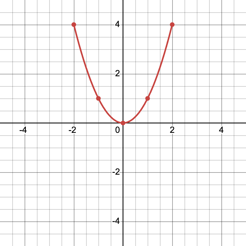
Example 1: Consider the parameters and . Let .
- Create the table:
| -2 | -2 | 4 |
| -1 | -1 | 1 |
| 0 | 0 | 0 |
| 1 | 1 | 1 |
| 2 | 2 | 4 |
- Plot and connect these: Observe a parabolic path opening upwards.
Understanding the Domain of Parametric Functions
The domain of parametric equations, concerning , influences where the graph starts and stops. For instance, a parameter restriction indicates a segment of the entire curve.
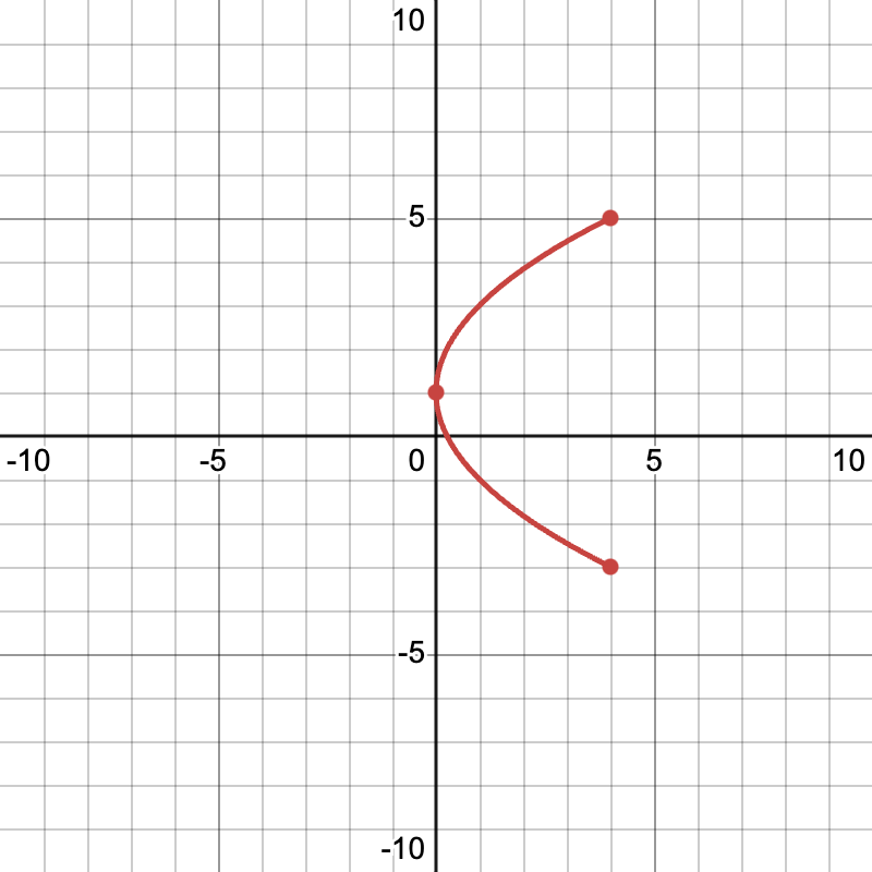
Analyze the domain of , for .
- The curve forms half a circle from the positive -axis to the negative one.
Exploring Different Types of Parametric Curves
Parametric equations can graph many curve types, like circles or ellipses.
- Circle: Use .
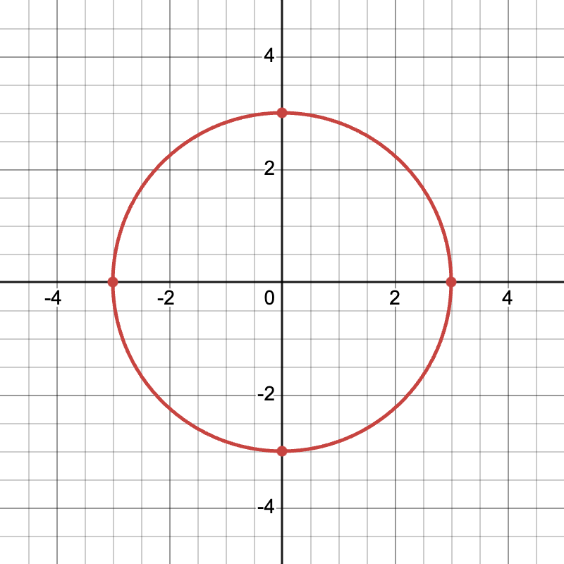
Example 3: Graph a circle with radius 3. The equations are , , running .
- The complete path forms a circle centered at the origin.
Using Parametric Equations in Real-World Applications
Parametric equations often model real-life scenarios, such as motion paths.
Example 4: Model a projectile’s path. Suppose , .
- Here, represents vertical motion influenced by gravity, while describes constant horizontal speed.
Quick Reference Chart
| Vocabulary | Definition/Key Feature |
| Parametric Equations | Equations defining x and y in terms of a parameter |
| Parameter | Independent variable controlling other variables |
| Domain | Range of values that determine the graph’s extent |
Conclusion
Mastering the graphs of parametric equations in Precalculus opens up many ways to visualize motion and trajectories. This understanding is vital for real-world applications and deeper mathematical exploration. Keep practicing these concepts for a solid foundation and explore more complex scenarios. Happy graphing!
Sharpen Your Skills for AP® Precalculus
Are you preparing for the AP® Precalculus exam? We’ve got you covered! Try our review articles designed to help you confidently tackle real-world math problems. You’ll find everything you need to succeed, from quick tips to detailed strategies. Start exploring now!
- 3.14 Polar Function Graphs
- 3.15 Rates of Change in Polar Functions
- 4.2 Parametric Functions Modeling Planar Motion
Need help preparing for your AP® Precalculus exam?
Albert has hundreds of AP® Precalculus practice questions, free responses, and an AP® Precalculus practice test to try out.


