Logistic growth describes how a population or quantity increases rapidly at first but levels off over time due to limitations. This behavior is common in real-life situations, such as bacterial growth in a dish or the spread of a rumor. The logistic growth differential equation captures this effect by including a factor that prevents the population from growing beyond a certain limit, known as the carrying capacity.

When modeling, it is useful to keep in mind that after some point, growth slows down because resources or space start to become scarce. Therefore, the main goal of the logistic growth differential equation is to show how a population adjusts as it approaches its maximum possible size. The main ideas you’ll see throughout this article are “logistic growth differential equation,” “logistic models with differential equations,” and “graph of carrying capacity.”

The standard form of the logistic growth differential equation is written as:

\frac{d(y)}{dt} = k y \bigl(a - y\bigr)

Here, y is the population (or quantity), a is the carrying capacity, and k is a constant that measures how quickly growth takes place.

Basic Concepts of Logistic Growth

Carrying Capacity

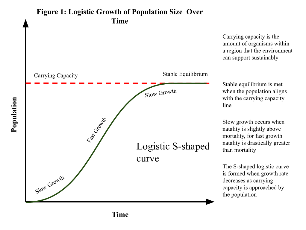
Carrying capacity is the maximum number or value that an environment or system can sustain. If a population tries to go beyond this number, lack of resources or environmental constraints will cause the growth to slow down or even reverse.

• As the population y approaches the carrying capacity a, the term \bigl(a - y\bigr) in the logistic growth differential equation gets smaller.
• Eventually, the population stops growing once it hits the carrying capacity.

In the graph of carrying capacity concept, the curve will flatten near a, illustrating how population size levels off in the long run.

Rate of Growth and Proportionality

The rate of change \frac{d(y)}{dt} is proportional to two main factors:

1. The current quantity y.
2. The difference between the carrying capacity and the current quantity \bigl(a - y\bigr).

The constant k affects how fast the population moves toward the carrying capacity. When k is large, the population grows quickly before leveling off.

Understanding the Logistic Growth Differential Equation

Logistic models with differential equations view populations in a balance between growth and limitation. The full equation:

\frac{d(y)}{dt} = k y \bigl(a - y\bigr)

can be read part by part:

• y represents the current size of the population.
• a - y shows how much room is left before reaching the maximum size.
• k controls how effectively the population uses the remaining space to grow.

Initial conditions, such as y(0) = y_0, are needed to understand how the population starts and then evolves over time. Even without solving the equation fully, it is possible to interpret whether the population is growing or shrinking at any point by noting if (a - y) is positive or negative.

Example 1: Interpreting the Logistic Equation Without Solving

Problem Statement:

Consider the logistic growth differential equation:

\frac{d(y)}{dt} = k y\bigl(a - y\bigr)

Suppose k, a, and the initial condition y(0) = y_0 are known. How can the direction of growth be determined without finding the full solution?

Step-by-Step Interpretation:

1. Check whether y(t) < a.

• If y is less than a, then (a - y) is positive. Because y is also positive, the product k y(a - y) is positive. Therefore, the population is increasing.

2. Check whether y(t) > a.

• If y were larger than a, then (a - y) would be negative. This would make \frac{d(y)}{dt} negative, suggesting the population decreases toward the carrying capacity.

3. As t \to \infty, note that y(t) approaches a.

• Because the growth rate slows down near a, y(t) will settle around the carrying capacity in the long run.

Key Takeaways

• When y(t) is below the carrying capacity, the population grows.
• When y(t) is above the carrying capacity, the population decreases.
• Long-term population size stabilizes at a.

Fastest Rate of Change in Logistic Models

Concept Overview

A striking feature of logistic models with differential equations is that the population experiences its fastest growth when it is exactly halfway to the carrying capacity. Intuitively, there is enough population to reproduce quickly, yet there is still plenty of room to grow.

Example 2: Finding the Point of Maximum Growth

Problem Statement:

Given \frac{d(y)}{dt} = k y \bigl(a - y\bigr), find the value of y at which the rate of growth is the greatest.

Step-by-Step Solution:

1. Recognize that the rate of growth is \frac{d(y)}{dt}.
2. Notice that \frac{d(y)}{dt} = k y\bigl(a - y\bigr) will be largest (in the positive range) where y maximizes the product y (a - y).
3. Rewrite y (a - y) = a y - y^2. The maximum of this expression occurs where the two factors are balanced.
4. Set y = \frac{a}{2}. At this point, the population is half of the carrying capacity.

Discussion

This result implies that the population’s fastest growth rate happens when there is an ideal balance between available space and the number of individuals. A larger population takes up more room, reducing the growth. A smaller population lacks enough individuals to reproduce at the maximum pace. Therefore, y = \frac{a}{2} is the “sweet spot” for the highest rate of change.

Quick Reference Chart

Term	Definition
Logistic Growth Differential Equation	An equation that models population growth with a limiting factor, written as \frac{d(y)}{dt} = k y (a - y).
Logistic Models with Differential Equations	Mathematical frameworks used to study populations or quantities that approach a carrying capacity.
Carrying Capacity	The maximum population or value an environment or system can sustain.
Rate Constant k	A constant that determines the speed of growth in the logistic model.
Initial Condition	The starting value of the population or quantity at a certain time, used to solve or interpret the model.

Conclusion

The logistic growth differential equation provides a powerful way to understand how populations evolve under resource limits. It shows that growth initially increases quickly but eventually slows near the carrying capacity a. In addition, the fastest rate of change occurs at half of that carrying capacity. These insights hold true in many practical settings, from biology to economics.

Logistic models with differential equations continue to be essential for studying real-world problems where a system cannot increase without bound. Observing the graph of carrying capacity in theory offers clarity on how populations tend to stabilize over time. Understanding these principles helps in predicting long-term behavior and making informed decisions in fields like conservation, resource management, and public health.

Sharpen Your Skills for AP® Calculus AB-BC

Are you preparing for the AP® Calculus exam? We’ve got you covered! Try our review articles designed to help you confidently tackle real-world math problems. You’ll find everything you need to succeed, from quick tips to detailed strategies. Start exploring now!

Need help preparing for your AP® Calculus AB-BC exam?

Albert has hundreds of AP® Calculus AB-BC practice questions, free responses, and an AP® Calculus AB-BC practice test to try out.