Mean Value Theorem (MVT): AP® Calculus AB-BC Review

The mean value theorem is an important principle in calculus that connects average rate of change to instantaneous rate of change. Many students preparing for AP® Calculus AB-BC wonder, “what is the mean value theorem?” In short, the MVT says that under certain conditions, there is a point in an interval where the function’s derivative equals the function’s average rate of change. This concept is central to understanding deeper topics in mvt calculus and beyond.

Why the Mean Value Theorem Matters

Many find the MVT fascinating because it links two core ideas: average rate of change and instantaneous rate of change. Suppose a person travels along a straight road. The average rate of change calculates the overall speed from start to finish, but the MVT guarantees there is at least one moment along the way when the exact speed matches that average. Therefore, it helps form a bridge between the broader, overall behavior of a function and its precise behavior at specific points. This principle appears in many real-life motion problems in calculus.

Conditions for the MVT

The mean value theorem has two key requirements. These conditions must be met over the specified interval.

Continuity on [a, b]

Continuity over [a, b] means the function has no jumps or breaks on that interval. A continuous function is one where all points from x = a to x = b connect smoothly. Therefore, no gaps exist in the interval [a, b].

Differentiability on (a, b)

Differentiability on (a, b) ensures that the derivative exists at each point inside the open interval. For a function to be differentiable, it must be smooth enough that a tangent line can be drawn at every point between a and b. Thus, a function that meets both conditions is ready for an MVT analysis.

Formal Statement of the MVT

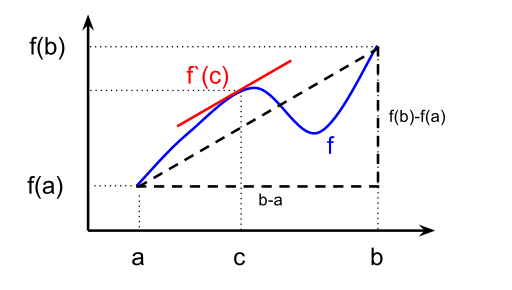
The formal statement of the mean value theorem says: if a function f(x) is continuous on [a, b] and differentiable on (a, b), then there exists at least one point c in (a, b) such that

\frac{f(b) - f(a)}{b - a} = f'(c).

Because both conditions hold, the theorem guarantees that this special point c exists. Therefore, the average rate of change from x=a to x=b matches the instantaneous rate of change at x=c.

Step-by-Step Example 1

Consider a simple polynomial function f(x) = x^2 on the interval [1, 3]. This problem meets the MVT conditions because polynomials are continuous and differentiable everywhere.

1. Check continuity and differentiability:
   • Polynomials have no breaks or gaps, so x^2 is continuous for all x.
   • The derivative, f'(x) = 2x, exists for all x. Thus, x^2 is differentiable on (1, 3).
2. Calculate the average rate of change from x=1 to x=3: \frac{f(3) - f(1)}{3 - 1} = \frac{(3)^2 - (1)^2}{2} = \frac{9 - 1}{2} = \frac{8}{2} = 4.
3. Set the derivative equal to the average rate of change to find c: The derivative is f'(x) = 2x. So, solve 2x = 4.Therefore, x = 2.

Hence, c=2 is the point where the instantaneous rate of change matches the average rate of change on [1, 3].

Practice Problem: Try verifying the mean value theorem for f(x)=x^3 from x=0 to x=2.

1. Check that f(x)=x^3 is continuous on [0,2] and differentiable on (0,2).
2. Compute the average rate of change: \frac{f(2)-f(0)}{2-0}.
3. Set f'(x)=3x^2 equal to that average rate of change. Solve for x in (0,2).

Step-by-Step Example 2

Now consider f(x)=\sin(x) on [0, \pi]. This example offers practice with a trigonometric function.

1. Verify conditions for the MVT:
   • \sin(x) is continuous on the closed interval [0, \pi].
   • It is differentiable on the open interval (0, \pi) since \frac{d}{dx}(\sin x)=\cos x exists everywhere.
2. Find the average rate of change on [0, \pi]: \frac{\sin(\pi) - \sin(0)}{\pi - 0} = \frac{0 - 0}{\pi} = 0.
3. Solve f'(x)=\cos(x) = average rate of change. In other words, \cos(x) = 0. Between 0 and \pi, this happens at x = \frac{\pi}{2}.

Thus, c=\frac{\pi}{2} is a point where the instantaneous rate of change (\cos(x)) matches the average rate of change (0).

Practice Problem: Apply the MVT to f(x)=\tan(x) on \left[\frac{\pi}{4}, \frac{3\pi}{4}\right].

1. Check continuity and differentiability on the specified interval.
2. Find \frac{f\left(\frac{3\pi}{4}\right) - f\left(\frac{\pi}{4}\right)}{\frac{3\pi}{4}-\frac{\pi}{4}}.
3. Solve f'(x)=\sec^2(x) = average rate of change.

Common Pitfalls and Misconceptions

Sometimes a function is continuous but not differentiable at every point in the interval. If differentiability fails on (a, b), the mean value theorem may not apply. Another related theorem is Rolle’s Theorem, which is often confused with the MVT. However, Rolle’s Theorem is a special case that applies when f(a)=f(b). It is also a mistake to ignore endpoints or to forget that c must exist strictly between a and b when checking the MVT. Therefore, always confirm the two key conditions before proceeding.

Quick Reference Chart

Vocabulary	Definition/Explanation
Mean Value Theorem (MVT)	If f is continuous on [a, b] and differentiable on (a, b), then there exists a c in (a, b) where the instantaneous rate of change equals the average rate of change.
Average Rate of Change	\frac{f(b) - f(a)}{b - a}; the slope of the secant line over [a, b].
Instantaneous Rate of Change	f'(x); the derivative, or slope of the tangent line.
Continuous Function	A function with no breaks or gaps on an interval.
Differentiable Function	A function whose derivative exists on an interval.

Conclusion

The mean value theorem offers a guarantee that on any interval where the function is both continuous and differentiable, a point exists where the instantaneous rate of change equals the average rate of change. Indeed, the MVT clarifies “what is the mean value theorem” and demonstrates the power of calculus to connect broad interval-based information to specific moments in a function’s behavior. By mastering these ideas, students gain a greater understanding of mvt calculus and build a strong foundation for more advanced topics. Readers are encouraged to explore additional examples and practice problems to become even more comfortable with the MVT’s applications.

Sharpen Your Skills for AP® Calculus AB-BC

Are you preparing for the AP® Calculus exam? We’ve got you covered! Try our review articles designed to help you confidently tackle real-world math problems. You’ll find everything you need to succeed, from quick tips to detailed strategies. Start exploring now!

Need help preparing for your AP® Calculus AB-BC exam?

Albert has hundreds of AP® Calculus AB-BC practice questions, free responses, and an AP® Calculus AB-BC practice test to try out.