Introduction

Graphs full of scattered dots may look messy at first. However, the SAT® loves these pictures because a scatter plot and its model help translate real-world data into clear predictions. Whenever two numerical variables interact (temperature versus ice-cream sales, time versus distance) a scatterplot can capture the story in seconds. Therefore, anyone aiming for a high SAT® Math score must know how to read the pattern, fit the right model, and interpret what the slope or curve actually means.

Quick Warm-Up: What a Scatterplot Shows

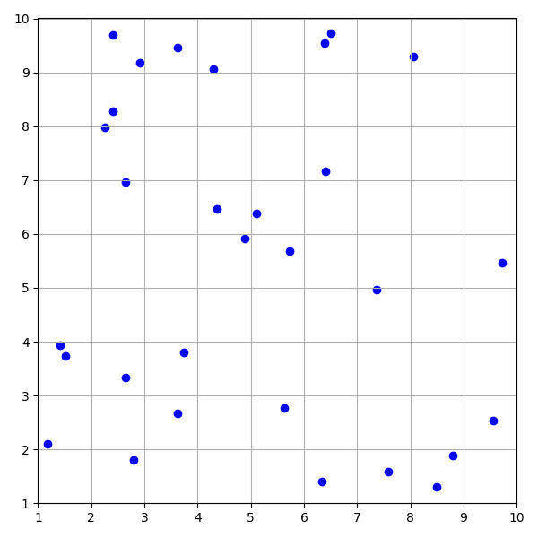
A scatterplot is a graph of ordered pairs. Each dot represents one measurement of two quantitative variables.

• The horizontal axis (x) shows the independent variable.
• The vertical axis (y) shows the dependent variable.

On the SAT®, questions built on a simple dot graph often ask students to:

• Identify the trend
• Choose or write an equation that fits the data
• Use the model to predict future points

Because the dots show actual data, the overall direction, shape, and any unusual points all matter.

Spotting Patterns at a Glance

Quick visual checks save time.

A. Direction

• Positive association: dots rise from left to right.
• Negative association: dots fall from left to right.
• No association: dots look random.

B. Clusters and Outliers

• Clusters suggest sub-groups.
• Outliers sit far from the main cloud and can pull trend lines away from the true center.

C. Straight or Curved Trend

Sometimes the dots hug a straight path; other times they bend. Deciding early whether a line or a curve is best sets up every later step.

Example 1 — Reading a Scatterplot

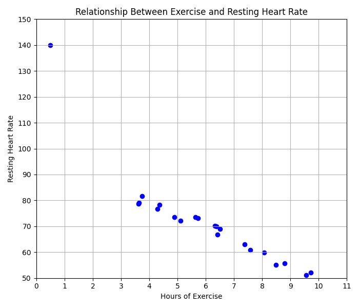
1. Read the axis titles: “Hours of Exercise” (x) and “Resting Heart Rate” (y).
2. Dots decrease from left to right and are close together. Therefore, the association is negative and fairly strong.
3. One point at (0.5, 140) sits far above the others. That outlier could raise the best-fit line and lessen the negative slope.

The Line of Best Fit: Sketching, Calculating, and Interpreting

A. Estimating Slope

Pick two anchor points on the imagined trend line. Then use rise over run.

m=\dfrac{\text{change in }y}{\text{change in }x}

B. Finding the y-Intercept

Extend the line left until it meets the y-axis. That height is the intercept b.

C. Technology Tip

The SAT® sometimes provides regression output such as y = 2.6x + 4.1. Knowing how to read those numbers is faster than recomputing by hand.

Example 2 — Building an Equation

A scatterplot of “cups of coffee (x)” vs. “hours awake (y)” looks linear.

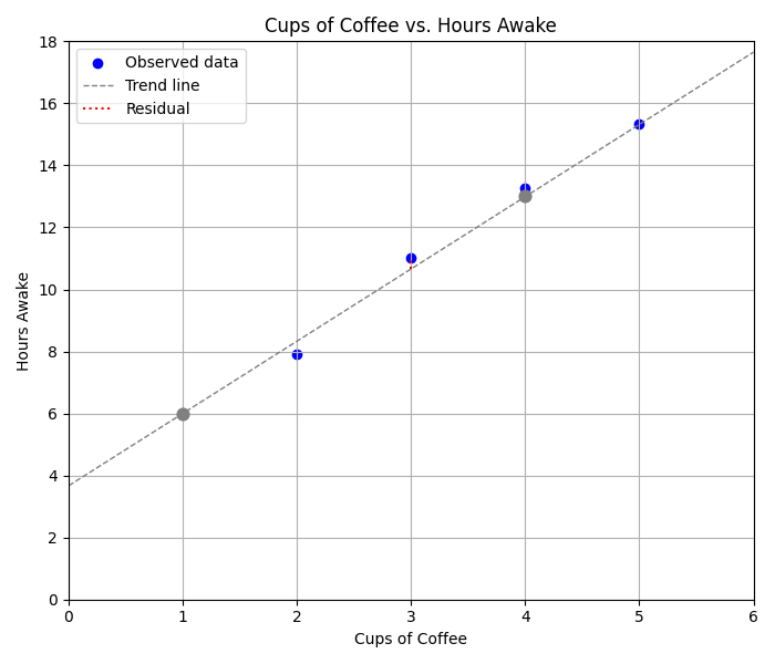
1. Draw a light trend line.
2. Choose two points on the line, say (1, 6) and (4, 13).
3. Calculate slope:
   • m=\dfrac{13-6}{4-1}= \dfrac{7}{3}\approx2.33
   • Use point-slope form:
     • y-6 = 2.33(x-1)
   • Simplify:
     • y = 2.33x + 3.67

Prediction Check: For 3 cups, predicted hours are:

y = 2.33(3)+3.67 \approx 10.66

The actual dot at x = 3 shows 11 hours, so the residual is about 0.34, which is quite small.

Slope and Intercept in Context

A slope tells the rate of change. Therefore, it answers “How much does y grow (or fall) when x increases by one?”

An intercept gives the starting value when x = 0.

Example 3 — Interpretation

Given y = 2.3x + 5 for “hours studied (x) vs. test score increase (y)”

• Slope 2.3 means each extra hour adds about 2.3 points to the score.
• Intercept 5 means a student who studies zero hours still gains 5 points—perhaps from regular class time.

Beyond Straight Lines: Selecting Linear, Quadratic, or Exponential Models

A. Linear

• Constant difference pattern (add 3, add 3…).
• Dots align roughly straight.

B. Quadratic

• One bend; looks like a U or upside-down U.
• Second differences stay constant.

C. Exponential

• Curve increases or decreases more and more quickly.
• Multiplicative pattern (\cdot 1.5, \cdot 1.5…).

Example 4 — Data Table Identification

x	y_1	y_2	y_3
0	2	5	1
1	5	4	2
2	8	-1	4
3	11	-10	8
4	14	-23	16

• y_1 adds 3 each step → Linear.
• y_2 subtracts 1 then 5 then 9 → Second differences constant at −4 → Quadratic.
• y_3 multiplies by 2 each step → Exponential.

Linear vs. Exponential Growth—Side-by-Side

Linear growth adds the same amount. Exponential growth multiplies by the same factor. Therefore, exponential always overtakes linear in the long run.

Example 5 — Graph Comparison

Plot y = 3x + 2 and y = 2\cdot(1.5)^x for 0 \le x \le 6.

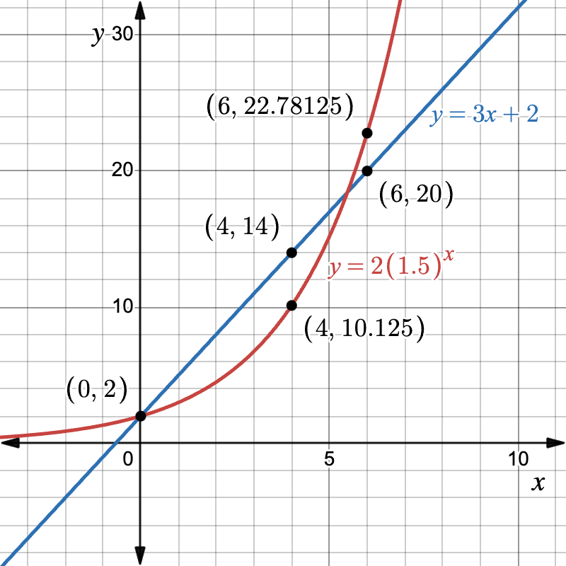
• At x = 0, linear gives 2; exponential gives 2.
• At x = 4, linear gives 14; exponential gives about 10.1.
• At x = 6, linear gives 20; exponential gives about 22.8 and has passed the line.

Thus, exponential growth eventually wins.

Using a Model for Prediction and Reasonableness Checks

• Interpolation: predicting inside the plotted x-range.
• Extrapolation: predicting beyond it; riskier because the pattern might change.

A residual reveals error:

\text{residual}= \text{actual }y - \text{predicted }y

Example 6 — Predicting and Checking

The best-fit equation for “years since purchase (x)” vs. “car value in \$1{,}000 (y)” is y = 18 - 1.5x.

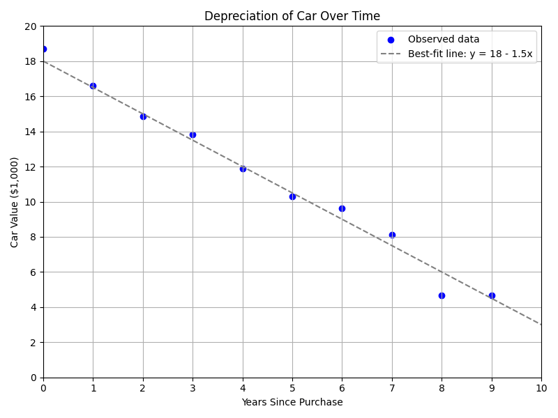
1. Predict the value after 7 years:
   • y = 18 - 1.5(7) = 7.5 thousand dollars.
2. The actual data point shows \$8.1 k.
   • Residual = 8.1 − 7.5 = 0.6 (in thousands).
3. Because 0.6 is small relative to the car price, the model seems reasonable at x = 7.

Common SAT® Traps and Time-Saving Tips

• Watch axis units; sometimes one square = 5 units.
• Keep x and y in order while computing slope; mixing them reverses the sign.
• Avoid wild extrapolation. The SAT® often places answer choices that assume a trend far outside the data range.

Quick Reference Chart

Term	Definition	SAT® Tip
Scatterplot	Graph of ordered pairs showing two-variable data	Look at the overall trend first
Line of best fit	Straight line that minimizes total residuals	Can be estimated visually
Slope	Change in y per 1-unit change in x	Represents “rate” in word problems
y-intercept	y value when x = 0	Often, the initial amount
Residual	Actual y − Predicted y	Smaller = better fit
Linear growth	Adds a constant amount	Straight trend
Exponential growth	Multiplies by a constant factor	The curve gets steeper
Quadratic model	Parabolic curve with one turning point	Check for symmetry

Quick Practice Set

1. A scatterplot shows a positive linear trend with estimated equation y = 0.8x + 12. Predict y when x = 15.
2. The table (x, y) = (0, 4), (1, 12), (2, 36), (3, 108) most likely fits what model type?
3. The residual for a data point is −5. What does the negative sign tell about the actual y-value compared to the prediction?

Answer Key

1. y = 0.8(15)+12 = 24
2. Exponential (tripling each time).
3. Actual y-value is 5 units below the model’s prediction.

Final Takeaways

Scatterplots and models unlock quick points on test day. First, recognize the pattern and choose a sensible model. Next, interpret slope and intercept in context, then use the equation to make smart predictions. Consistent practice—both with hand-drawn sketches and calculator regression—turns these steps into automatic wins under timed conditions.

Sharpen Your Skills for SAT® Math (Digital)

Are you preparing for the SAT® Math (Digital) test? We’ve got you covered! Try our review articles designed to help you confidently tackle real-world SAT® Math (Digital) problems. You’ll find everything you need to succeed, from quick tips to detailed strategies. Start exploring now!

Need help preparing for your SAT® Math (Digital) exam?

Albert has hundreds of SAT® Math (Digital) practice questions, free response, and full-length practice tests to try out.